How to use the GROUPBY function 13 Oct 2024 1:09 AM (last year)
What is the GROUPBY function?
The GROUPBY function allows you to aggregate data through a formula vertically. It is a formula-based alternative to the traditional pivot table for many summarizing operations. The function is a dynamic array formula and is only available to Excel 365 subscribers.
Table of Contents
- Introduction
- Syntax
- Example 1 - create totals by category
- Example 2 - aggregate by category and sort from large to small
- Example 3 - summarize by two categories
- Example 4 - create totals by year
- Example 5 - aggregate by year and month
- Example 6 - summarize by year and quarter
- Example 7 - create totals by year and week
- Example 8 - create totals and count in the same column
- Example 9 - aggregate values and sort by count
- Example 10 - aggregate values and display corresponding invoice numbers
- Extract unique distinct values sorted based on sum of adjacent values - Excel 365
- Extract unique distinct values sorted based on sum of adjacent values - earlier Excel versions
- Filtering unique distinct text values and sorting them based on the sum of adjacent values and criteria - earlier Excel versions
- Filtering unique distinct text values and sorting them based on the sum of adjacent values and criteria - Excel 365
1. Introduction
What is a dynamic array formula?
A dynamic array formula in Excel 365 is a type of formula that can return multiple values which are then automatically spills into a range of adjacent cells below and/or to the right. This allows for more flexible and dynamic calculations as the formula can adapt to the size of the data. Dynamic array formulas in Excel 365 are entered as regular formulas in contrast to array formulas in older Excel versions that required you to press CTRL + SHIFT + ENTER.
What is spilling?
Spilling in Excel 365 refers to the process of a formula returning multiple values, which are then automatically displayed in a range of cells. This is a key feature of dynamic array formulas, as it allows the formula to adapt to the size of the data and display the results in a flexible and dynamic way. When a formula spills, the values are displayed in a range of cells, and the formula is denoted by a blue border.
What is aggregating values?
Aggregating values in Excel refers to the process of combining multiple values into a single value often using a mathematical operation such as sum, average, or count. Aggregating values is a common task in data analysis, as it allows you to summarize and analyze large datasets.
What is a pivot table?
A pivot table in Excel is a powerful data analysis tool that allows you to summarize and analyze large datasets.
- A pivot table is a table that can be rotated and manipulated to display different views of the data allowing you to easily summarize and analyze the data from different angles.
- Pivot tables are particularly useful for analyzing large datasets as they allow you to quickly and easily summarize and analyze the data, and to create custom views of the data.
- Pivot tables can be used to perform a variety of tasks, including aggregating values, filtering data, and creating custom reports.
The GROUPBY function allows for aggregating values in rows or vertically. How can I aggregate values also in columns or horizontally?
The PIVOTBY function allows for summarizing for both rows (vertically) and columns (horizontally).
What are the benefits of using the GROUPBY function instead of using a Pivot Table?
- You can analyze text values as well. This is not possible with the Pivot Table.
- Changes in the source data is immediately shown in the formula output. This is not the case with Pivot Tables, you need to refresh the Pivot Table in order to calculate new aggregated values.
2. Syntax
GROUPBY(row_fields, values, function, [field_headers], [total_depth], [sort_order], [filter_array], [field_relationship])
| Argument | Text |
| row_fields | Required. The fields that determines the aggregated values. You may use multiple fields. |
| values | Required. The data you want to aggregate. |
| function | Required. The function that is used to aggregate values.
SUM: The sum of a range of cells. |
| [field_headers] | Optional. A number between 0 (zero) and 3, if missing automatic mode which is the default. Automatic determines if the data source contains headers based on their data type text or number. Missing: Automatic. (default) 0: No 1: Yes and don't show 2: No but generate 3: Yes and show |
| [total_depth] | Optional. This specifies if the row headers should disply totals.
Missing: Automatic: Grand totals and, where possible, subtotals. (default) |
| [sort_order] | Optional. A number that corresponds to the columns in the row_fields argument. A positive number and the rows are sorted in ascending order, a negative numbers sorts the rows in descending order. |
| [filter_array] | Optional. A logical expression that evaluates to TRUE or FALSE which indicates if the corresponding value is included in the calculation. |
| [field_relationship] | Optional. A number:
0: Hierarchy (defualt) sorting takes into account the hierarchy of earlier columns. 1: Sorting is done independently. Subtotals are not supported. |
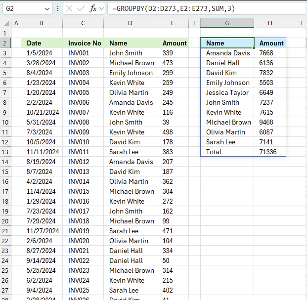
3. Example 1 - aggregate based on item
This example demonstrates how to aggregate values based on items, in this case, names. The output array contains header names. The image above shows an Excel spreadsheet containing invoice numbers (source data) and a summary table. The main table (columns A-E) has the following columns: Date, Invoice No, Name, Amount. It lists various transactions with dates ranging from 2024, invoice numbers (INV001-INV031), customer names, and corresponding amounts.
The formula shown in the formula bar is the contents of cell G2:
The arguments are:
- row_fields - D2:D273 The column header name is included in the cell reference.
- values - E2:E273 The column header name is included in the cell reference.
- function - SUM
- [field_headers] - 3 representing "Yes, and show".
To the right (columns F-G) is a summary table that is generated using a GROUPBY function. This table shows:"Name" and "Amount" The Amount column in the summary table is the total amount for each unique name from the main table. At the bottom of this summary, there's a "Total" row showing the total of all aggregated amounts.
This summary is created by grouping the data from the main table by name and aggregating the amounts for each person. This spreadsheet tracks financial transactions or sales by individual with the summary providing a quick overview of total amounts per person.
4. Example 2 - aggregate based on item and sort
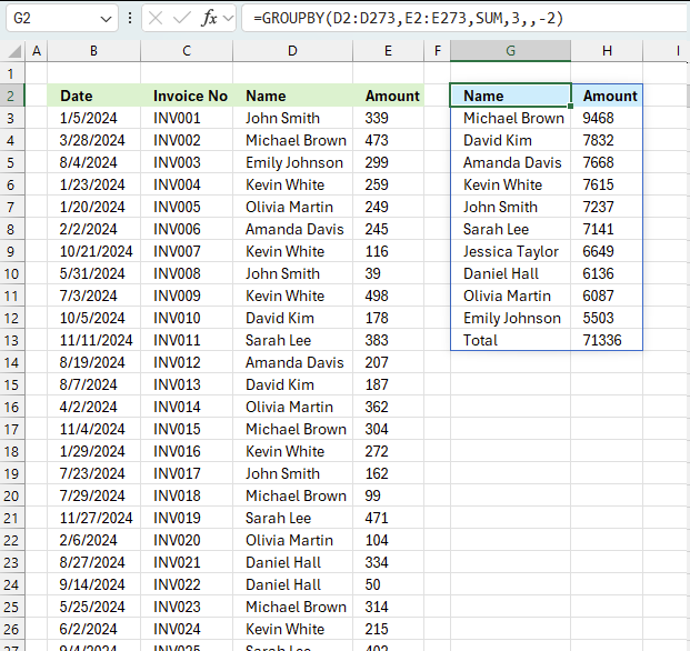
This example shows how to summarize sales amounts based on names, the output is sorted based on output column in descending order meaning from large to small.
The source data is in cell range B3:E273, it contains 4 columns with header names Date, Invoice No, Name, and the corresponding amount.
The formula shown in the formula bar is the contents of cell G2:
The arguments are:
- row_fields - D2:D273 The column header name is included in the cell reference.
- values - E2:E273 The column header name is included in the cell reference.
- function - SUM
- [field_headers] - 3 representing "Yes, and show".
- [sort_order] - -2 meaning the output array is sorted based on column 2 in descending order.
The image above shows the output array in cell range G2:H13.
5. Example 3 - aggregate based on two items
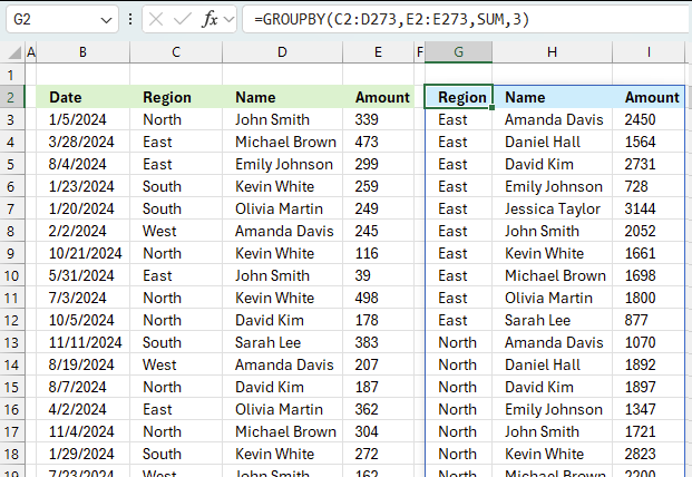
This example shows how to summarize numbers based on two categories, in this case "Region" and "Name". The amounts on the same row corresponds to the "Region" and "Name". The source data is in cell range B3:E273, it contains the following columns: "Date", "Region", "Name", and "Amount".
The arguments are:
- row_fields - D2:D273 The column header name is included in the cell reference.
- values - E2:E273 The column header name is included in the cell reference.
- function - SUM
- [field_headers] - 3 representing "Yes, and show".
Note that the cell references contain the column header names as well. This allows you to show the column names if 3 is specified in the fourth argument named [field_headers] which tells the function to display the included column header names.
The difference between this example and example 1 above is that the first argument contains two columns instead of one. The output array contains both these columns, however, duplicate rows are merged into one distinct row.
6. Example 4 - aggregate based on year
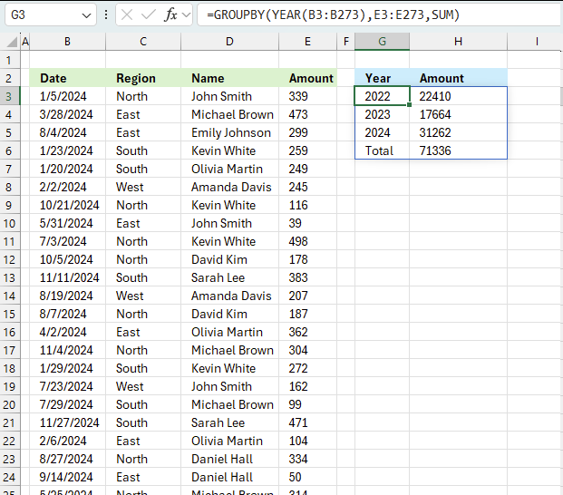
The image above shows the function in cell G3. the column header names above are hard coded meaning they are actual typed values and not the result of a formula. The source data is in cell range B3:E273, it contains the following columns: "Date", "Region", "Name", and "Amount".
The arguments are:
- row_fields - YEAR(B3:B273) The column header name is not included in the cell reference.
- The YEAR function returns the year based on an Excel date. It has the following syntax: YEAR(serial)
Serial is the actual Excel date or in this case multiple Excel dates.
- The YEAR function returns the year based on an Excel date. It has the following syntax: YEAR(serial)
- values - E3:E273 The column header name is included in the cell reference.
- function - SUM
The output array, displayed in cell G3 and adjacent cells below and to the right, summarizes the amounts based on the corresponding year based on the specified date in column "Date".
- YEAR(B3:B273): This part extracts the year from dates in the range B3:B273. It creates a array of years, which will be used as the grouping criteria.
- E3:E273: This is the range of values to be summarized which is the "Amount" column in the data set.
- SUM: This is the operation to be performed on the grouped data.
What this formula does:
- It groups the data by year (extracted from column B).
- For each unique year, it sums the corresponding values from column E.
The result will be a summary table showing:
- Unique years from column B
- Total sum of amounts (from column E) for each year
This formula is useful for creating an annual summary of financial data, showing the total amount for each year represented in the dataset.
7. Example 5 - aggregate based on year and month

This example demonstrated in the image above shows the function in cell G3. the column header names above are hard coded meaning they are actual typed values and not the result of a formula. The source data is in cell range B3:E273, it contains the following columns: "Date", "Region", "Name", and "Amount".
The arguments are:
- row_fields - TEXT(B3:B273,"yyyy-mmm") The column header name is not included in the cell reference.
- The TEXT function returns the year and month based on an Excel date in column B. It has the following syntax: TEXT(value, format_code)
Value is the actual Excel date or in this case multiple Excel dates.
- The TEXT function returns the year and month based on an Excel date in column B. It has the following syntax: TEXT(value, format_code)
- values - E3:E273 The column header name is included in the cell reference.
- function - SUM
The output array, displayed in cell G3 and adjacent cells below and to the right, summarizes the amounts based on the corresponding year and month based on the specified date in column "Date".
- TEXT(B3:B273,"yyyy-mmm") : This part extracts the year and month from dates in the range B3:B273. It creates a array of years and months, which will be used as the grouping criteria.
- E3:E273: This is the range of values to be summarized which is the "Amount" column in the data set.
- SUM: This is the operation to be performed on the grouped data.
What this formula does:
- It groups the data by year and month extracted from column B.
- For each unique year and month, it sums the corresponding values from column E.
The result will be a summary table showing:
- Unique years and months from column B
- Total sum of amounts (from column E) for each year
This formula is useful for creating an monthly summary of financial data, showing the total amount for each month represented in the dataset.
8. Example 6 - aggregate values based on year and quarter
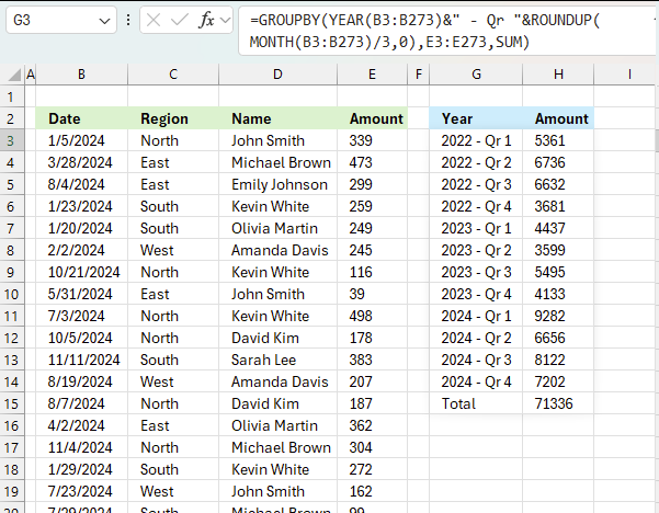
This example demonstrates how to aggregate values based on year and quarter using the GROUPBY function in cell G3. The column header names above are hard coded meaning they are actual typed values and not the result of a formula. The source data is in cell range B3:E273, it contains the following columns: "Date", "Region", "Name", and "Amount".
The arguments are:
- row_fields - YEAR(B3:B273)&" - Qr "&ROUNDUP(MONTH(B3:B273)/3,0) The column header name is not included in the cell reference.
- The YEAR function returns the year based on an Excel date in column B. It has the following syntax: YEAR(serial).
- The ampersand character & concatenates values.
- ROUNDUP(MONTH(B3:B273)/3,0) calculates the quarter number.
- values - E3:E273 The column header name is included in the cell reference.
- function - SUM
The output array, displayed in cell G3 and adjacent cells below and to the right, summarizes the amounts based on the corresponding year and quarter calculated based on the specified date in column "Date".
- YEAR(B3:B273): Extracts the year from the dates in the range B3:B273.
- MONTH(B3:B273): Extracts the month number (1-12) from the dates in the range B3:B273.
- MONTH(B3:B273)/3 Divides the month number by 3.
- ROUNDUP(..., 0): Rounds up the result of the division to the nearest integer, effectively giving us the quarter number. This gives a decimal value representing the quarter:
- Months 1-3 (Q1): result 1
- Months 4-6 (Q2): result 2
- Months 7-9 (Q3): result 3
- Months 10-12 (Q4): result 4
- " - Qr ":A literal string that will separate the year from the quarter in the final output.
- &: The ampersands concatenate all these parts into a single string.
The complete formula YEAR(B3:B273)&" - Qr "&ROUNDUP(MONTH(B3:B273)/3,0) will produce results like:
"2024 - Qr 1" for dates in January, February, or March 2024
"2024 - Qr 2" for dates in April, May, or June 2024
"2024 - Qr 3" for dates in July, August, or September 2024
"2024 - Qr 4" for dates in October, November, or December 2024
This formula is useful for grouping dates by both year and quarter, which can be helpful for financial reporting or seasonal analysis of data.
What this formula does:
- It groups the data by year and quarter extracted from column B.
- For each unique year and quarter, it sums the corresponding values from column E.
The result will be a summary table showing:
- Unique years and quarters from column B
- Total sum of amounts (from column E) for each year
This formula is useful for creating an quarterly summary of financial data, showing the total amount for each quarter represented in the dataset.
9. Example 7 - aggregate values based on year and week

This example demonstrates how to aggregate values based on year and week number using the GROUPBY function in cell G3. The column header names above are hard coded meaning they are actual typed values and not the result of a formula. The source data is in cell range B3:E273, it contains the following columns: "Date", "Region", "Name", and "Amount".
Formula in cell G3:
The arguments are:
- row_fields - HSTACK(YEAR(B3:B273),BYROW(B3:B273,LAMBDA(a,WEEKNUM(a,1)))) The column header name is not included in the cell reference.
- values - G3:G273 The column header name is not included in the cell reference.
- function - SUM
The output array is shown in cell I3 and adjacent cells to the right and below. It displays aggregated amounts based on year and week number specified in column B and C.
Here is a quick break down of the formula:
- HSTACK: This function horizontally combines arrays or values.
Inside HSTACK, we have two arguments:- YEAR(B3:B273):
- This extracts the year from each date in the range B3:B273.
- It creates a single-column array of years.
- The WEEKNUM function does not allow an array of values, we need a workaround. The BYROW function lets us use a cell range as an input value.
BYROW(B3:B273,LAMBDA(a,WEEKNUM(a,1))):- BYROW applies a function to each row of the given range.
- The LAMBDA function defines what to do for each row:
WEEKNUM(a,1) calculates the week number of the date in each row.
The ",1" in WEEKNUM meaning week begins on Sunday.
- YEAR(B3:B273):
- GROUPBY(HSTACK(...),E3:E273,SUM): This aggregates values in E3:E273 based on the given year and week numbers
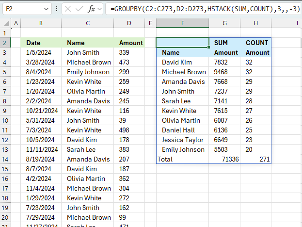
10. Example 8 - aggregate values and display sum and count
This example shows how to aggregate numbers and show the corresponding count meaning how many values are included in each summary. The down side is that you want be able to sort the values since they now are text values. The first value shown in cell G3 is "Amanda Davis", the sum is 7668 shown in cell H3 and after the hyphen "-" the total number of indivdual numbers in sum sum are shown. In this case, 29 numbers are included in the sum of 7668.
The formula in cell G2:
This formula uses the GROUPBY function in Excel along with a LAMBDA function to create a custom summary. Let's break it down:
- D2:D273 - This is the first argument of GROUPBY and represents the column to group by, likely the "Name" column in your data.
- E2:E273 - This is the second argument, representing the values to summarize, likely the "Amount" column.
- LAMBDA(a,SUM(a)&"-"&COUNT(a)) - This is a custom aggregation function:
- LAMBDA(a, ...) defines an anonymous function where 'a' represents each group of values.
- SUM(a) calculates the total sum for each group.
- COUNT(a) counts the number of items in each group.
- & "-" & concatenates the sum and count with a hyphen between them.
- 3: This argument specifies that header names will be shown.
The result of this formula will be a summary table with:
- Column 1: Unique names from column D
- Column 2: A string in the format "Sum-Count" for each name, where:
- Sum is the total amount for that name
- Count is the number of entries for that name
For example, if John Smith had 3 invoices totaling $1000, his row in the summary might look like: John Smith | 1000-3 |
This formula provides a concise summary of both the total amount and the number of transactions for each unique name in your dataset.
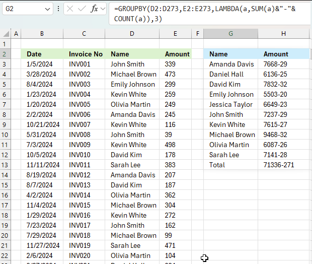
11. Example 9 - aggregate values and sort by count
Example 8 above showed how to display both the sum and the count for each category, however, this made it hard to sort the values as both values concatenated in the same cell creates a text string. This example shows how to build a formula that creates both the amount and the count in different columns which enables sorting based on the count.
Formula in cell F3:
The arguments are:
- row_fields - C2:C273 The column header name is included in the cell reference.
- values - C2:C273 The column header name is included in the cell reference.
- function - HSTACK(SUM,COUNT) - The HSTACK function allows for multiple functions, all in different columns. This example demonstrates SUM and COUNT functions.
- [field_headers] - 3 representing "Yes, and show".
- [sort_order] - -3 meaning sort on the third column (COUNT) from large to small
12. Example 10 - aggregate values and display corresponding invoice numbers
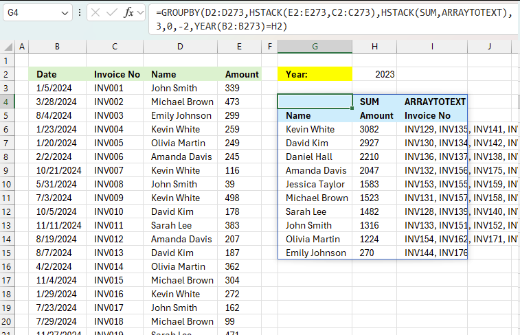
This example shows how to:
- filter values using the [filter_array] argument based on year specified in yellow cell H2
- aggregate amounts based on names in column H
- sort the totals in descending order meaning from large to small
- display corresponding invoice numbers horizontally in columns I and adjacent columns to the right
all in one formula
Excel 365 dynamic array formula in cell G4:
The arguments in the GROUPBY function are:
- row_fields - D2:D273 The column header name is included in the cell reference.
- values - HSTACK(E2:E273,C2:C273) The column header name is included in the cell reference. The HSTACK function allows for multiple columns, in this case, both the values and invoice numbers.
- function - HSTACK(SUM,ARRAYTOTEXT): The HSTACK function allows for multiple functions as well, in this case, both aggregate and text values.
- 3 - show column header names
- 0 - no grand total
- -2 - sort values based on column 2 (aggregated numbers) from large to small
- YEAR(B2:B273)=H2 - filter values if date in column B is in the same year as specified in cell H2
13. Extract unique distinct values sorted based on sum of adjacent values - Excel 365

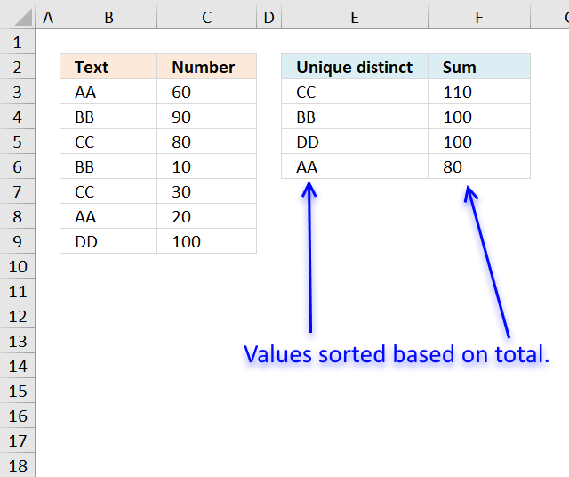
This example demonstrates a formula that lists unique distinct values in column B and returns a sorted list based on the totals in column C from large to small.
Value "CC" is displayed in cells C5 and C7, they are 80 and 30 respectively, and the total is 110.
Value "BB" is displayed in cells C4 and C6, they are 90 and 10 respectively, and the total is 100.
Value "DD" is displayed in cell C9, the value is 100, and the total is 100.
Value "AA" is displayed in cells C3 and C7, they are 60 and 20 respectively, and the total is 80.
Update! New function in Excel 365!
Excel 365 dynamic array formula in cell E3:
Read more about the GROUPBY function.
Excel 365 dynamic array formula:
Formula in cell F3:
Explaining formula
Step 1 - Extract unique distinct values
The UNIQUE function returns a unique or unique distinct list.
Function syntax: UNIQUE(array,[by_col],[exactly_once])
UNIQUE(B3:B9)
becomes
UNIQUE({"AA";"BB";"CC";"BB";"CC";"AA";"DD"})
and returns
{"AA";"BB";"CC";"DD"}.
Step 2 - Calculate totals based on the unique list
The SUMIF function sums numerical values based on a condition.
Function syntax: SUMIF(range, criteria, [sum_range])
SUMIF(B3:B9,UNIQUE(B3:B9),C3:C9)
becomes
SUMIF({"AA";"BB";"CC";"BB";"CC";"AA";"DD"}, {"AA";"BB";"CC";"DD"}, {60;90;80;10;30;20;100})
and returns
{80;100;110;100}
Step 3 - Sort totals from largest to smallest
The SORTBY function sorts a cell range or array based on values in a corresponding range or array.
Function syntax: SORTBY(array, by_array1, [sort_order1], [by_array2, sort_order2],…)
SORTBY(UNIQUE(B3:B9),SUMIF(B3:B9,UNIQUE(B3:B9),C3:C9),-1)
becomes
SORTBY({"AA";"BB";"CC";"DD"},{60;90;80;10;30;20;100},-1)
and returns
{"CC";"BB";"DD";"AA"}.
Step 4 - Shorten the formula
The LET function lets you name intermediate calculation results which can shorten formulas considerably and improve performance.
Function syntax: LET(name1, name_value1, calculation_or_name2, [name_value2, calculation_or_name3...])
SORTBY(UNIQUE(B3:B9),SUMIF(B3:B9,UNIQUE(B3:B9),C3:C9),-1)
y - B3:B9
x - UNIQUE(y)
LET(y,B3:B9,x,UNIQUE(y),SORTBY(x,SUMIF(y,x,C3:C9),-1))
14. Extract unique distinct values sorted based on the sum of adjacent values - earlier Excel versions
This formula is for earlier Excel versions.
Array formula in E2:
How to create an array formula
- Copy above array formula
- Double press with left mouse button on cell E3
- Paste array formula
- Press and hold Ctrl + Shift simultaneously
- Press Enter
Formula in cell F3:
Explaining formula in cell E2
Step 1 - Count prior values above the current cell
The COUNTIF function counts values based on a condition or criteria, if the number is 0 (zero) then the corresponding value has not yet been displayed.
NOT(COUNTIF($D$1:D1, $A$2:$A$8))
becomes
NOT(COUNTIF("Unique distinct", {"AA";"BB";"CC";"BB";"CC";"AA";"DD"}))
becomes
NOT({0;0;0;0;0;0;0})
The NOT function returns the boolean opposite to the given argument. The array contains no boolean values, however it does contain their numerical equivavents. TRUE = 1 and FALSE = 0 (zero).
NOT({0;0;0;0;0;0;0})
and returns
{TRUE; TRUE; TRUE; TRUE; TRUE; TRUE; TRUE}.
Step 2 - IF TRUE then return the corresponding sum
The IF function returns the total if the boolean value is TRUE. FALSE returns "" (nothing).
IF(NOT(COUNTIF($E$2:E2, $B$3:$B$9)),SUMIF($B$3:$B$9, "="&$B$3:$B$9, $C$3:$C$9),"")
becomes
IF({TRUE; TRUE; TRUE; TRUE; TRUE; TRUE; TRUE}, SUMIF($B$3:$B$9, "="&$B$3:$B$9, $C$3:$C$9),"")
The SUMIF function adds numbers and returns a total based on a condition or criteria.
IF({TRUE; TRUE; TRUE; TRUE; TRUE; TRUE; TRUE}, SUMIF($B$3:$B$9, "="&$B$3:$B$9, $C$3:$C$9),"")
becomes
IF({TRUE; TRUE; TRUE; TRUE; TRUE; TRUE; TRUE}, {80;100;110;100;110;80;100},"")
and returns
{80;100;110;100;110;80;100}.
Step 3 - Get the largest number in array
The MAX function returns the largest number in the array ignoring blanks and text values.
MAX(IF(NOT(COUNTIF($E$2:E2, $B$3:$B$9)),SUMIF($B$3:$B$9, "="&$B$3:$B$9, $C$3:$C$9),""))
becomes
MAX({80;100;110;100;110;80;100})
and returns 110.
Step 4 - Match number
The MATCH function returns the relative position of a value in a cell range or array.
MATCH(MAX(IF(NOT(COUNTIF($E$2:E2, $B$3:$B$9)),SUMIF($B$3:$B$9, "="&$B$3:$B$9, $C$3:$C$9),"")), IF(NOT(COUNTIF($E$2:E2, $B$3:$B$9)),SUMIF($B$3:$B$9, "="&$B$3:$B$9, $C$3:$C$9),""), 0)
becomes
MATCH(110, IF(NOT(COUNTIF($E$2:E2, $B$3:$B$9)),SUMIF($B$3:$B$9, "="&$B$3:$B$9, $C$3:$C$9),""), 0)
becomes
MATCH(110, {80;100;110;100;110;80;100}, 0)
and returns 3.
Step 5 - Get value
The INDEX function returns a value based on row number (and column number if needed)
INDEX($A$2:$A$8, MATCH(MAX(IF(NOT(COUNTIF($D$1:D1, $A$2:$A$8)),SUMIF($A$2:$A$8, "="&$A$2:$A$8, $B$2:$B$8),"")), IF(NOT(COUNTIF($D$1:D1, $A$2:$A$8)),SUMIF($A$2:$A$8, "="&$A$2:$A$8, $B$2:$B$8),""), 0))
becomes
INDEX($A$2:$A$8, 3)
and returns "CC" in cell E2.
Get Excel *.xlsx file
Filter unique distinct list sorted based on sum of adjacent values.xlsx
15. Filtering unique distinct text values and sorting them based on the sum of adjacent values and criteria - earlier Excel versions

This formula is for earlier Excel versions than Excel 365. It extracts values based on the list specified in cells E1 and E2, the formula returns the list sorted based on totals of the adjacent numbers.
Array formula in cell E7:
Formula in cell E7:
Get excel *.xlsx file
filter-unique-distinct-list-sorted-based-on-sum-of-adjacent-values-using-array-formula2.xlsx
16. Filtering unique distinct text values and sorting them based on the sum of adjacent values and criteria - Excel 365

This formula is the same as in section 1 with one difference, values must be in the criteria list in order to be displayed.
Update!
The following formula demonstrates the new GROUPBY function, it has the following arguments:
- row_fields - B3:B9 (text values)
- values - C3:C9 (Numbers)
- function - SUM (Calculates totals based on numbers)
- [field_headers] - 0 (zero) - no column headers
- [total_depth]- 0 - no totals
- [sort_order]- -2 - sort based on column 2 in descending order
- [filter_array] - COUNTIF(F2:F3,B3:B9) - Filter values based on criteria specified in cells F2:F3
Excel 365 formula:
Excel 365 dynamic array formula in cell E6:
Formula in cell F6:
Explaining formula
Step 1 - Count values based on criteria
The COUNTIF function calculates the number of cells that is equal to a condition.
Function syntax: COUNTIF(range, criteria)
COUNTIF(F2:F3,B3:B9)
becomes
COUNTIF({"AA";"BB"},{"AA";"BB";"cc";"EE";"cc";"F F";"DD"})
and returns
{1; 1; 0; 0; 0; 0; 0}.
Step 2 - Filter values based on the count
The FILTER function extracts values/rows based on a condition or criteria.
Function syntax: FILTER(array, include, [if_empty])
FILTER(B3:B9,COUNTIF(F2:F3,B3:B9))
becomes
FILTER({"AA";"BB";"cc";"EE";"cc";"F F";"DD"},{1; 1; 0; 0; 0; 0; 0})
and returns
{"AA";"BB"}.
Step 3 - Extract unique distinct values
The UNIQUE function returns a unique or unique distinct list.
Function syntax: UNIQUE(array,[by_col],[exactly_once])
UNIQUE(FILTER(B3:B9,COUNTIF(F2:F3,B3:B9)))
becomes
UNIQUE({"AA";"BB"})
and returns
{"AA";"BB"}.
Step 4 - Calculate totals based on the unique list
The SUMIF function sums numerical values based on a condition.
Function syntax: SUMIF(range, criteria, [sum_range])
SUMIF(B3:B9,UNIQUE(FILTER(B3:B9,COUNTIF(F2:F3,B3:B9))),C3:C9)
becomes
SUMIF({"AA";"BB";"cc";"EE";"cc";"F F";"DD"}, {"AA";"BB"}, {60;90;80;-100;30;-50;0})
and returns
{60;90}.
Step 5 - Sort totals from largest to smallest
The SORTBY function sorts a cell range or array based on values in a corresponding range or array.
Function syntax: SORTBY(array, by_array1, [sort_order1], [by_array2, sort_order2],…)
SORTBY(UNIQUE(FILTER(B3:B9,COUNTIF(F2:F3,B3:B9))),SUMIF(B3:B9,UNIQUE(FILTER(B3:B9,COUNTIF(F2:F3,B3:B9))),C3:C9),-1)
becomes
SORTBY({"AA";"BB"},{60;90},-1)
and returns
{"BB";"AA"}.
Step 6 - Shorten the formula
The LET function lets you name intermediate calculation results which can shorten formulas considerably and improve performance.
Function syntax: LET(name1, name_value1, calculation_or_name2, [name_value2, calculation_or_name3...])
SORTBY(UNIQUE(FILTER(B3:B9,COUNTIF(F2:F3,B3:B9))),SUMIF(B3:B9,UNIQUE(FILTER(B3:B9,COUNTIF(F2:F3,B3:B9))),C3:C9),-1)
y - B3:B9
x - UNIQUE(FILTER(y,COUNTIF(F2:F3,y)))
LET(y,B3:B9,x,UNIQUE(FILTER(y,COUNTIF(F2:F3,y))),SORTBY(x,SUMIF(y,x,C3:C9),-1))


Complex Calculations: A Guide to Excel’s IM Functions 19 Mar 2024 10:58 PM (2 years ago)
Table of Contents
- How to use the IMABS function
- How to use the IMAGINARY function
- How to use the IMARGUMENT function
- How to use the IMCONJUGATE function
- How to use the IMCOS function
- How to use the IMCOSH function
- How to use the IMCOT function
- How to use the IMCSC function
- How to use the IMCSCH function
- How to use the IMDIV function
- How to use the IMEXP function
- How to use the IMLN function
- How to use the IMLOG10 function
- How to use the IMLOG2 function
- How to use the IMPOWER function
- How to use the IMPRODUCT function
- How to use the IMREAL function
- How to use the IMSEC function
- How to use the IMSECH function
- How to use the IMSIN function
- How to use the IMSINH function
- How to use the IMSQRT function
- How to use the IMSUB function
- How to use the IMSUM function
- How to use the IMTAN function
- How to use the COMPLEX function
1. How to use the IMABS function

The IMABS function calculates the absolute value (modulus) of a complex number in x + yi or x + yj text format.
A complex number consists of an imaginary number and a real number, complex numbers let you solve polynomial equations using imaginary numbers if no solution is found with real numbers. It has applications in engineering such as electronics, electromagnetism, signal analysis, and more.
Table of Contents
1.1. Syntax
IMABS(inumber)
1.2. Arguments
| inumber | Required. A complex number in x+yi or x+yj text format. |
1.3. Example
The IMABS function calculates the modulus of a complex number, IMABS probably stands for imaginary absolute. The absolute value is the same as the modulus.
The modulus of a complex number is the distance of the complex number from the origin in the complex plane. It is the square root of the sum of the squares of the real part and the imaginary part of the complex number. If the complex number is Z then the modulus is denoted |Z|.
The image above shows a chart of the complex plane, complex number 9+12i is the blue line ending with an arrow. The complex plane has an imaginary axis and a real axis, the dashed circle shows the modulus value when it crosses both the imaginary axis and the real axis.
Formula:
The formula calculates the modulus based on the value in cell C26 which is "9+12i" in this example. The formula returns 15 which the dashed circle also shows when it crosses the imaginary and real axis. Section 4 below explains in greater detail how the IMABS function calculates the modulus.
The modulus is needed when you want to:
- convert complex numbers from rectangular form to polar form or vice versa.
- compare sizes or magnitudes of different complex numbers.
- calculate the distance between two complex numbers
1.3.1 Explaining formula
Step 1 - Populate arguments
IMABS(inumber)
becomes
IMABS(C26)
Step 2 - Evaluate IMABS function
IMABS(C26)
becomes
IMABS("9+12i")
and returns 15.
1.4. How is the modulus calculated in detail?

The formula to calculate the absolute value or modulus z from a complex number is based on the Pythagorean theorem.
z2 = x2+y2
The IMABS function calculates the absolute value using this formula which is based on the Pythagorean theorem:
IMABS(z) = |z| =√(x2+y2)
x is the real coefficient and y is the imaginary coefficient of the complex number.
The modulus of a complex number is how far it is from the point where the real and imaginary axes cross (0,0). It is the square root of the real part squared plus the imaginary part squared.
Here is how the modulus is calculated for complex number 9+12i:
z = x + yi
z = 9 + 12i
IMABS(z) = |z| =√(x2+y2)
IMABS(z) = |z| =√(92+122)
IMABS(z) = |z| =√(81+144)
IMABS(z) = |z| =√225
IMABS(z) = |z| =15
1.5. How imaginary numbers were invented
1.6. How to convert complex numbers to polar form?

Formula in cell D4:
Complex numbers are usually presented in this form
z = x + yi
or
z = x + yj
However, complex numbers can also be represented in polar form:
z = r*(cos θ + isin θ)
In other words, theta θ in the polar form is calculated using the IMARGUMENT based on complex numbers.
Pythagorean Theorem
r2 = x2 + y2
To calculate the absolute value we can use this formula:
r = √(x2+y2)
Excel has a function that does this for you, the IMABS function calculates the absolute value based on complex numbers.
Explaining formula
Step 1 - Calculate theta θ
The IMARGUMENT function calculates theta θ which is an angle displayed in radians based on complex numbers in rectangular form.
Function syntax: IMARGUMENT(inumber)
IMARGUMENT(C4)
becomes
IMARGUMENT("12+9i")
and returns
0.643501108793284
Step 2 - Calculate the absolute value
The IMABS function calculates the absolute value (modulus) of a complex number in x + yi or x + yj text format.
Function syntax: IMABS(inumber)
IMABS(C4)
becomes
IMABS("12+9i")
and returns
15
Step 3 - Join calculations with text
The ampersand character lets you concatenate values in an Excel Formula.
IMABS(C4)&"(cos "&IMARGUMENT(C4)&" + isin "&IMARGUMENT(C4)&")"
Step 4 - Evaluate the formula
IMABS(C4)&"(cos "&IMARGUMENT(C4)&" + isin "&IMARGUMENT(C4)&")"
becomes
15&"(cos "&0.643501108793284&" + isin "&0.643501108793284&")"
and returns
15(cos 0.643501108793284 + isin 0.643501108793284)
Useful links
2. How to use the IMAGINARY function

The IMAGINARY function calculates the imaginary number of a complex equation in x + yi or x + yj text format.
The letter j is used in electrical engineering to distinguish between the imaginary value and the electric current.
Table of Contents
2.1. Syntax
IMAGINARY(inumber)
2.2. Arguments
| inumber | Required. A complex number in x+yi or x+yj text format. |
2.3. Example
A complex number consists of an imaginary number and a real number, complex numbers let you solve polynomial equations using imaginary numbers if no solution is found with real numbers.
A complex number in rectangular form can be described as z = x + yi or z = x + yj text form in Excel. The IMAGINARY function extracts the imaginary value from the complex number.
Formula in cell D3:
The imaginary coefficient is the number ending with a i or j, this number is what the IMAGINARY function extracts from a complex number.
2.3.1 Explaining formula
Step 1 - Populate arguments
IMAGINARY(inumber)
becomes
IMAGINARY(B25)
Step 2 - Evaluate IMAGINARY function
IMAGINARY(C3)
becomes
IMAGINARY("3+4i")
and returns 4.
2.4. When to use the IMAGINARY function?
Use the IMAGINARY function when you want to
- add, subtract, multiply and divide complex numbers.
- calculate the modulus which is the distance from the origin to the point representing the complex number.
- graph complex numbers
- calculate the complex determinant of a 2x2 matrix
The links above points to articles explaining how to manually calculate these properties, however, Excel has functions so you don't need to calculate them manually:
IMSUM | IMSUB | IMPRODUCT | IMDIV | IMARGUMENT | IMABS
2.5. How to plot the imaginary part of a complex number on a chart
The chart above shows how to represent the complex number “3+4i” on the complex plane. The complex plane has two axes: the x-axis is for real numbers and the y-axis is for imaginary numbers. The blue line with an arrow points from the origin (0,0) to (3,4), which is the location of “3+4i” on the plane.
The horizontal dashed line marks the imaginary part of the complex number “3+4i” on the y-axis. The IMAGINARY function can extract the real part from any complex number, which is useful for plotting complex numbers on charts.
A complex number has both a real part and an imaginary part, and we need both of them to plot a complex number on the plane.
2.5.1 Calculate the real and imaginary parts of a complex number

To plot a complex number on the complex plane, we have to find its real and imaginary parts separately. Cell B25 has the complex number in rectangular form.
Formula in cell C25:
The IMREAL function extracts the real number from the complex number in cell B25.
Formula in cell D25:
The IMAGINARY function extracts the imaginary number from the complex number in cell B25.
To plot a line, we need to use coordinates from the origin (0,0), so I have entered 0 (zero) in cells C24 and D24. The scatter chart that we will create soon requires a blank row between the line coordinates to show two separate lines that are not connected.
The dashed line also needs two points on the chart to be displayed correctly. It starts from where the complex number is (3,4) and ends at the y-axis. The line is horizontal, so the end point must have an real part of 0 (zero).
2.5.2 Insert a scatter chart

The following steps describe how to plot a complex number and the corresponding real number.
- Select cell range C24:D28.
- Go to tab "Insert" on the ribbon.
- Press with left mouse button on the "Insert Scatter (x,y) or Bubble chart" button.

- A popup menu appears, press with left mouse button on the "Scatter with straight lines".
A chart shows up on the worksheet, move the chart to its desired location.
Change the chart so it shows the complex number as a line with an ending arrow, the imaginary number as a dashed line and so on. Here are detailed instructions:
How to plot theta θ - Argand diagram
Useful links
IMAGINARY function - Microsoft
3. How to use the IMARGUMENT function

The IMARGUMENT function calculates the argument theta θ which is an angle displayed in radians based on complex numbers in rectangular form like z = x + yi or z = x + yj.
Table of Contents
3.1. Syntax
IMARGUMENT(inumber)
3.2. Arguments
| inumber | Required. A complex number in x+yi or x+yj text format. |
3.3. Example
The image above shows how to calculate the θ with the IMARGUMENT function based on the corresponding complex numbers on the same row specified in cell B3. The dashed circle represents the complex modulus |z| of "2+3i" and the angle theta represents its complex argument.
Formula in cell C3:
The IMARGUMENT function returns a value expressed in radians, the image above shows a chart where theta θ is displayed in degrees.
3.3.1 Explaining formula
Step 1 - Populate arguments
IMARGUMENT(inumber)
becomes
IMARGUMENT(B3)
Step 2 - Evaluate IMARGUMENT function
IMARGUMENT(B3)
becomes
IMARGUMENT("2+3i")
and returns
0.982793723247329
3.4. How is the theta θ calculated in detail?
The IMARGUMENT function calculates theta θ expressed in radians using this formula:
θ = tan-1(y/x) for x>0
Here is how 0.982793723247329 is calculated:
tan θ = y/x
becomes
θ = tan-1(y/x)
tan-1(y/x)
becomes
tan-1(3/2)
equals
0.982793723247329
3.5. How to convert angle theta θ from radians to degrees
The following formula calculates theta θ based on a given complex number in rectangular form, the result is a value expressed in radians.
The DEGREE function takes the radian value and converts it to degrees.
Formula:
3.5.1 Explaining formula
Step 1 - Calculate theta θ in radians
The IMARGUMENT function calculates theta θ which is an angle displayed in radians based on complex numbers in rectangular form.
Function syntax: IMARGUMENT(inumber)
IMARGUMENT(B3)
becomes
IMARGUMENT("2+3i")
and returns
0.982793723247329
Step 2 - Convert radians to degrees
The DEGREES function calculates degrees from radians.
Function syntax: DEGREES(angle)
DEGREES(IMARGUMENT(B3))
becomes
DEGREES(0.982793723247329)
and returns
56.3099324740202
3.6. How to plot theta θ - Argand diagram

The image above shows an Argand diagram which is a chart of complex numbers, the dashed circle is the modulus of the complex numbers.
C1 = 2 +3i
|C1| = |2 +3i| = Modulus = square root of 13 = 3.605551
theta θ = tan-1(3/2) = 0.982793723247329 radians = 56.3099324740202 degrees
Change the complex number in cell B31 and the chart adjusts accordingly.
3.6.1 Calculate the numbers
We need to setup the worksheet before we can insert the scatter chart.

Value in cells C24, D27, C30, and D30: 0
Formula in cell D24, D25, D28, and D31:
Formula in cell C25. C27, C28, and C31:
Value in cell D27: 0
Value in cells C30 and D30: 0
Formula in cell B33:
3.6.2 Explaining formula in cell B33
The value in cell B33 will be used in the chart, I will show you how to do that below.
Step 1 - Calculate theta θ
The ATAN function calculates the arctangent of a number.
Function syntax: ATAN(number)
ATAN(D31/C31)
Step 2 - Convert radians to degree
The ATAN function calculates the arctangent of a number.
Function syntax: ATAN(number)
DEGREES(ATAN(D31/C31))
Step 3 - Round degrees to one digit
The ATAN function calculates the arctangent of a number.
Function syntax: ATAN(number)
ROUND(DEGREES(ATAN(D31/C31)),1)
Step 4 - Concatenate values
"θ: "&ROUND(DEGREES(ATAN(D31/C31)),1)&"°"
3.6.3 Create values for a circle on the chart

The following formulas in cells C33 and D33 calculates values that creates a circle on the chart, the image above shows a circle on a chart.
Formula in cell C33:
3.6.4 Explaining formula in cell C33
Step 1 - Calculate each 15 degree segment
The PI function returns the number pi (¶).
Function syntax: PI()
PI()/12
Step 2 - Create a sequence
The ROWS function calculate the number of rows in a cell range.
Function syntax: ROWS(array)
ROWS($A$1:A1)-1
Step 3 - Multiply segment with sequence
The ROWS function calculate the number of rows in a cell range.
Function syntax: ROWS(array)
PI()/12*(ROWS($A$1:A1)-1)
Step 4 - Calculate sine
The SIN function calculates the sine of an angle.
Function syntax: SIN(number)
SIN(PI()/12*(ROWS($A$1:A1)-1))
Step 5 - Calculate modulus
The IMABS function calculates the absolute value (modulus) of a complex number in x + yi or x + yj text format.
Function syntax: IMABS(inumber)
IMABS($B$31)
Step 6 - Multiply sine with modulus
SIN(PI()/12*(ROWS($A$1:A1)-1))*IMABS($B$31)
Formula in cell D33:
The formula in cell D33 is the same as in cell C33, except it calculates the cosine instead.
The cos function calculates the cosine of an angle.
Function syntax: COS(number)
Copy cells C33 and D33, paste to 24 rows below so the entire circle can be charted.
3.6.5 Insert "Scatter with smooth lines" chart
- Select cell range B24:D57.
- Go to tab "Insert" on the ribbon.
- Press with left mouse button on the "Scatter (x,y) or Bubble chart" button on the ribbon.
- A popup menu appears. Press with left mouse button on the "Scatter with smooth lines" button.
A new chart is now created. Move the chart to the desired location.

Select the chart, the boundaries now have "handles" that you can drag with the mouse to resize the chart.
- Double-press with left mouse button on the circle to select all lines on the chart and open the settings pane.

- Press with left mouse button on the "Fill & Line" button on the settings pane.
- Press with left mouse button on the "Line" on the settings pane, new settings in context to "Line" shows up.
- Press with left mouse button on the "Dash type" button, select a dashed line.

- All lines are now dashed. Press with left mouse button on the "Color" button and change to black.
3.6.6 Change the complex number line on the chart
- Select only the "complex number" line. Press with left mouse button on the "complex number" line once to select it if you have all lines selected.
If no lines are selected then press with left mouse button on the "complex number" line twice to select it. - Press with left mouse button on the "Line" on the settings pane. Change color, dash type and add an ending arrow.

- Repeat these steps for the imaginary and real lines.

Change the chart tite, use the settings pane to change the axis line widths and colors, remove chart grids.

- Select the "complex number" line (blue).
- Press with left mouse button on the "plus" sign next to the chart.

- Press with left mouse button on the check box next to "Data Labels" to enable data labels.
- Open the settings pane.
- Go to "Label options"

- Press with left mouse button on checkbox next to "Value From Cells", select cell B33.

- Move the data label to its destination.

Useful links
IMARGUMENT function - Microsoft
Argument of a complex number
What Is Argument Of Complex Number?
4. How to use the IMCONJUGATE function

The IMCONJUGATE function calculates the complex conjugate of a complex number in x + yi or x + yj text format.
The letter j is used in electrical engineering to distinguish between the imaginary value and the electric current.
Table of Contents
4.1. Syntax
IMCONJUGATE(inumber)
4.2. Arguments
| inumber | Required. A complex number in x+yi or x+yj text format. |
4.3. Example
The image above demonstrates a formula in cell D3 that calculates the complex conjugate of a complex number specified in cell C3. The chart shows the complex number 3+4i on the complex plane, it also shows the complex conjugate of 3+4i which is 3-4i.
Formula in cell D3:
4.3.1 Explaining formula
Step 1 - Populate arguments
IMCONJUGATE(inumber)
becomes
IMCONJUGATE(C3)
Step 2 - Evaluate IMCONJUGATE function
IMCONJUGATE(C3)
becomes
IMCONJUGATE("3+4i")
and returns
"3-4i".
4.4. How is the complex conjugate calculated?
The complex conjugate is calculated by changing the sign of the imaginary value of a complex number. The real part and the imaginary part are equal in magnitude however the imaginary part is opposite in sign.
IMCONJUGATE(x+yi) = z̄ = (x-yi)
The complex conjugate is often denoted as z̄.
Z = x+yi
z̄ = x-yi
4.5. How to calculate the product of a complex number and its complex conjugate

The product of a complex number and its conjugate is a real number.
z*z̄ = |z|^2
z*z̄ = (3+4i)*(3-4i) = 9-12i+12i+16 = 25
|z|^2 = 5^2 = 25
Formula in cell D3:
The image above shows a chart that has a complex number, its complex conjugate and the product plotted on a complex plane. The light blue line is the complex number, the green line is its complex conjugate and the orange line is the product of those two complex numbers.
4.5.1 Explaining formula in cell D3
Step 1 - Calculate the complex conjugate
The IMCONJUGATE function calculates the complex conjugate of a complex number in x + yi or x + yj text format.
Function syntax: IMCONJUGATE(inumber)
IMCONJUGATE(B25)
becomes
IMCONJUGATE("3+4i")
and returns
"3-4i"
Step 2 - Calculate the product of a complex number and its complex conjugate
The IMPRODUCT function calculates the product of complex numbers in x + yi or x + yj text format.
Function syntax: IMPRODUCT(inumber1, [inumber2], ...)
IMPRODUCT(B25,IMCONJUGATE(B25))
becomes
IMPRODUCT("3+4i","3-4i")
and returns 25.
4.6. How to calculate the modulus of a complex conjugate

The conjugate of a complex number z̄ has the same modulus as the complex number z.
|z̄| = |z|
The image above shows the modulus as a grey dashed circle on the chart, both the complex number and its complex conjugate has the same modulus.
Formula in cell C24:
IMABS(B24)
Formula in cell B25:
Formula in cell C25:
The formulas above also show that the modulus of a complex number is the same as the modulus of its complex conjugate. Cell C24 contains "3+4i", the complex conjugate is "3-4i" displayed in cell B25. The modulus is 5 for both the complex number and its complex conjugate.
4.7. How to calculate the conjugate of a conjugate complex number

The conjugate of a conjugate of a complex number is the original complex number,
Formula in cell D3:
The above formula demonstrates that it is the original complex number. Cell C3 contains the original complex number, cell D3 contains a formula that calculates the conjugate of a conjugate of the complex number in cell C3. The result is the exact same complex number.
Explaining formula
Step 1 - Calculate the complex conjugate
The IMCONJUGATE function calculates the complex conjugate of a complex number in x + yi or x + yj text format.
Function syntax: IMCONJUGATE(inumber)
IMCONJUGATE(C3)
becomes
IMCONJUGATE("3+4i")
and returns
"3-4i"
Step 2 - Calculate the complex conjugate
The IMCONJUGATE function calculates the complex conjugate of a complex number in x + yi or x + yj text format.
Function syntax: IMCONJUGATE(inumber)
IMCONJUGATE(IMCONJUGATE(C3))
becomes
IMCONJUGATE("3-4i")
and returns "3+4i"
Useful links
IMCONJUGATE function - Microsoft
Complex Conjugate
Complex conjugate - wikipedia
5. How to use the IMCOS function

What is the IMCOS function?
The IMCOS function calculates the cosine of a complex number in x + yi or x + yj text format.
The letter j is used in electrical engineering to distinguish between the imaginary value and the electric current.
What is the cosine?

The cosine is a trigonometric function that relates to an angle θ in a right triangle to the ratio of the length of the side adjacent the angle and the length of the longest side (hypotenuse) of the triangle. A right triangle has one angle that measures 90° or π/2 radians which is approximately 1.5707963267949 radians.
What is the difference between sine and the complex sine?
The difference between cosine and complex cosine is that the former is defined for real numbers only, while the latter is defined for complex numbers as well. The cosine of a complex number has some similarities to the cosine of a real number, such as periodicity.
The cosine function is periodic considering the angle, meaning it repeats its values after a certain interval. The period of the cosine function is 2π or 360 degrees.
cosine z = (eiz + e-iz)/2
z - complex number
i - imaginary unit
Table of Contents
5.1. Syntax
IMCOS(inumber)
5.2. Arguments
| inumber | Required. A complex number in x+yi or x+yj text format. |
5.3. Example
The image above demonstrates a formula in cell B28 that calculates the cosine of a complex number specified in cell B25.
Cell C28 calculates the real number from the complex number in cell B28. Cell D28 extracts the imaginary number from the complex number specified in cell B28.
The real and imaginary numbers separated in a cell each allow us to graph the complex number on the complex plane.
Formula in cell B28:
5.3.1 Explaining formula
Step 1 - Populate arguments
IMCOS(inumber)
becomes
IMCOS(B25)
Step 2 - Evaluate IMCOS function
IMCOS(B25)
becomes
IMCOS("2+2i")
and returns
-1.56562583531574-3.29789483631124i
5.4. How is the IMCOS function calculated in detail?
The cosine of a complex number is calculated like this:
C = x + yi
cos(C) = cos(x)*cosh(y) - sin(x)*sinh(y)i
For example, C=2+2i
cos(2+2i) = cos(2) cosh(2) - sin(2) sinh(2)i
becomes
cos(2+2i) = -0.416146836547142*3.76219569108363 + 0.909297426825682*3.62686040784702i
equals
cos(2+2i) = -1.56562583531574 - 3.29789483631124i
sin - calculates the sine of a number
cos - calculates the cosine of a number
cosh - calculates the hyperbolic cosine of a number
sinh - calculates the hyperbolic sine of a number
5.5. Function not working - #NUM error

The IMCOS function returns a #NUM error if the provided argument is not a valid complex number. The image above shows a worksheet with an invalid complex number specified in cell B25: 2+2
Excel needs an i or j in the complex number to work properly, correct the mistake and the IMCOS function will work again.
Useful links
IMCOS function - Microsoft
The Complex Cosine and Sine Functions - Mathonline
Cosine of Complex Number - Proofwiki
6. How to use the IMCOSH function

What is the IMCOSH function?
The IMCOSH function calculates the hyperbolic cosine of a complex number in x + yi or x + yj text format.
The letter j is used in electrical engineering to distinguish between the imaginary value and the electric current.
What is the hyperbolic cosine?
Hyperbolic functions are similar to ordinary trigonometric functions, but they use a different shape to define them.

Trigonometric functions use a circle, while hyperbolic functions use a hyperbola. The chart above shows a hyperbola and two asymptotes (dashed lines) where the intersection is at the center of the hyperbola. The chart below shows a circle containing the trigonometric functions.

What is a hyperbola?
The equation of a hyperbola with a horizontal axis is
(x2/ a2) - (y2 / b2) = 1
where a and b are positive constants.
A circle has a constant distance from the center point, while a hyperbola is a curve that has two focus points (+ae, 0), and (-ae, 0).
What is the difference between hyperbolic cosine and complex hyperbolic cosine?
The difference between hyperbolic cosine and hyperbolic cosine for complex numbers is that the former is defined for real numbers, while the latter is defined for complex numbers.
The hyperbolic cosine of a real number x is defined as
cosh(x) = (ex + e-x)/2
Natural number e is the base of the natural logarithm.
The complex hyperbolic cosine of a complex number z = x + yi is defined as cosh(z) = cosh(x)cos(y) + i sinh(x)sin(y)
Complex numbers has i as the imaginary unit.
Table of Contents
6.1. Syntax
IMCOSH(inumber)
6.2. Arguments
| inumber | Required. A complex number in x+yi or x+yj text format. |
6.3. Example
The image above demonstrates a formula in cell B28 that calculates the hyperbolic cosine of a complex number specified in cell B25.
Cell C28 calculates the real number from the complex number in cell B28. Cell D28 extracts the imaginary number from the complex number specified in cell B28.
The real and imaginary numbers separated in a cell each allow us to graph the complex number on the complex plane.
Formula in cell B28:
The chart above shows the complex plane, the y-axis is the imaginary axis and the x-axis is the real axis.
Complex number 2+i is the light blue line in the first quadrant. The hyperbolic cosine of 2+i is the green line also shown in the first quadrant.
6.3.1 Explaining formula
Step 1 - Populate arguments
IMCOSH(inumber)
becomes
IMCOSH(B25)
Step 2 - Evaluate the IMCOSH function
IMCOSH(B25)
becomes
IMCOSH("2+i")
and returns
2.03272300701967+3.0518977991518i
6.4. How the IMCOSH function is calculated in detail
The hyperbolic cosine of a complex number is calculated like this:
C = x + yi
cosh(x + yi) = cosh(x)*cos(y) + isinh(x)*sin(y)
For example, C=2+i
cosh(2 + i) = cosh(2)*cos(1) + isinh(2)*sin(1)
becomes
cosh(2 + i) = 3.76219569108363*0.54030230586814 + 3.62686040784702*0.841470984807897i
equals
cosh(2 + i) = 2.03272300701967+3.0518977991518i
6.5. Function not working

The IMCOSH function returns a #NUM error if the provided argument is not a valid complex number.
Useful links
IMCOSH function - Microsoft
Hyperbolic functions for complex numbers
Hyperbolic functions – Graphs, Properties, and Examples
Hyperbolic curve fitting in Excel
7. How to use the IMCOT function

The IMCOT function calculates the cotangent of a complex number in x + yi or x + yj text format.
The letter j is used in electrical engineering to distinguish between the imaginary value and the electric current.
What are complex numbers?
What is a cotangent?

The trigonometric cotangent is a function that relates an angle of a right-angled triangle to the ratio of adjacent side and the opposite side. It is also the inverse of the tangent, cot(θ) = 1/tan(θ).
What is the difference between cotangent and complex cotangent?
The difference between cotangent and cotangent for complex numbers is that the former is defined for real numbers, while the latter is defined for complex numbers.
The cotangent of a real number x is defined as cot(x) = i(eiθ + e-iθ)/(eiθ - e-iθ)
Natural number e is the base of the natural logarithm.
The complex cotangent of a complex number z = x + yi is defined as cot(x + yi) = (cosh(x)*cosh(y) - isin(x)*sinh(y)) / (sin(x)*cosh(y) + icos(x)*sinh(y))
Complex numbers has i as the imaginary unit.
Table of Contents
7.1. Syntax
IMCOT(inumber)
7.2. Arguments
| inumber | Required. A complex number in x+yi or x+yj text format. |
7.3. Example
The image above shows a formula in cell B28 that calculates the cotangent of a complex number specified in cell B25.
Cell C28 calculates the real number from the complex number in cell B28. Cell D28 extracts the imaginary number from the complex number specified in cell B28.
The real and imaginary numbers separated in a cell each allow us to graph the complex number on the complex plane.
Formula in cell B28:
The chart above shows the complex plane, the y-axis is the imaginary axis and the x-axis is the real axis.
Complex number 2+i is the light blue line in the first quadrant. The cotangent of 2+i is the green line located in the third quadrant.
7.3.1 Explaining formula
Step 1 - Populate arguments
IMCOT(inumber)
becomes
IMCOT(B25)
Step 2 - Evaluate the IMCOT function
IMCOT(C3)
becomes
IMCOT("2+i")
and returns
-0.171383612909185-0.821329797493852i
7.4. How is the IMCOT function calculated in detail?
The cotangent of a complex number is calculated like this:
cot(x + yi) = (cos(x)*cosh(y) - isin(x)*sinh(y)) / (sin(x)*cosh(y) + icos(x)*sinh(y))
For example, C=2+i
cot(2+i) = (cos(2)*cosh(1) - isin(2)*sinh(1)) / (sin(2)*cosh(1) + icos(2)*sinh(1))
becomes
cot(2+i) = (-0.416146836547142*1.54308063481524 - i0.909297426825682*1.1752011936438) / (0.909297426825682*1.54308063481524 + i-0.416146836547142*1.1752011936438)
becomes
cot(2+i) = (-0.64214812471552 - i1.06860742138278) / (1.40311925062204 + i-0.489056259041294)
equals
-0.171383612909184-0.821329797493853i
7.5. Function not working - #NUM error

The IMCOT function returns a #NUM error if the provided argument is not a valid complex number.
Useful links
IMCOT function - Microsoft
Cotangent of Complex Number
How to find cotangent of complex numbers
8. How to use the IMCSC function

The IMCSC function calculates the cosecant of a complex number in x + yi or x + yj text format.
The letter j is used in electrical engineering to distinguish between the imaginary value and the electric current.
What is a complex number?

A complex number contains a real and imaginary value, they let you for example solve equations with no real solutions like x2 + 1 = 0 The chart above shows x2 + 1 = 0 and it never touches the x-axis.
However, mathematicians invented the imaginary number and named it i, it extends into the complex plane and lets you solve equations using imaginary numbers.
What is the cosecant?
The cosecant is one of the six trigonometric functions, it is the multiplicative inverse of the sine function. This means that it is equal to 1 divided by the sine of a given angle θ.

The cosecant is csc θ = 1 / sin θ. In a right-angled triangle, the cosecant of an angle θ is equal to the hypotenuse divided by the opposite side.
What is the complex cosecant?
The complex cosecant is the extension of the cosecant function to the complex plane. It is defined as the reciprocal or the multiplicative inverse of the complex sine function, which means that it is equal to 1 divided by the sine of a complex number.
csc z = 1 / sin z, where z is a complex number.
The complex sine function can be expressed using the ordinary sine and cosine functions and the hyperbolic functions.
sin (x+yi) = sin x cosh y + i cos x sinh y
Table of Contents
8.1. Syntax
IMCSC(inumber)
8.2. Arguments
| inumber | Required. A complex number in x+yi or x+yj text format. |
8.3. Example
The image above demonstrates a formula in cell B28 that calculates the cosecant of a complex number specified in cell B25.
Cell C28 calculates the real number from the complex number in cell B28. Cell D28 extracts the imaginary number from the complex number specified in cell B28.
The real and imaginary numbers separated in a cell each allow us to graph the complex number on the complex plane.
Formula in cell D3:
The chart above shows the complex plane, the y-axis is the imaginary axis and the x-axis is the real axis.
Complex number 2+2i is the light blue line in the first quadrant. The cosecant of 2+2i is the small green line also displayed in the first quadrant.
8.3.1 Explaining formula
Step 1 - Populate arguments
IMCSC(inumber)
becomes
IMCSC(B25)
Step 2 - Evaluate the IMCSC function
IMCSC(B25)
becomes
IMCSC("2+2i")
and returns
0.244687073586957+0.107954592221385i
8.4. How is the IMCSC function calculated in detail?
The cosecant of a complex number is calculated like this:
C = x + yi
csc(C) = (sin(x)*cosh(y) - icos(x)*sinh(y)) / (sin²(x)*cosh²(y) + icos²(x)*sinh²(y))
For example, C = 2 + 2i
csc(2+2i) = (sin(2)*cosh(2) - icos(2)*sinh(2)) / (sin²(2)*cosh²(2) + icos²(2)*sinh²(2))
becomes
csc(2+2i) = (3.42095486111701 - (-1.50930648532362i)) / 13.9809382284401
equals
csc(2+2i) = 0.244687073586957+0.107954592221385i
8.5. IMCSC function not working

The IMCSC function returns a #VALUE! error if the argument is a boolean value.

The IMCSC function returns a #NUM! error if the argument is an invalid complex number. The i is missing in cell B25 shown in the image above.
Useful links
IMCSC function - Microsoft
Cosecant of Complex Number
Trigonometric functions - Wikipedia
9. How to use the IMCSCH function

What is the IMCSCH function?
The IMCSCH function calculates the hyperbolic cosecant of a complex number in x + yi or x + yj text format.
The letter j is used in electrical engineering to distinguish between the imaginary value and the electric current.
What is a complex number?
A complex number contains a real and imaginary value, they let you for example solve equations with no real solutions like x2 + 1 = 0 The chart above shows x2 + 1 = 0 and it never touches the x-axis.
However, mathematicians discovered the imaginary number i that solves equations into the complex plane.
What is the hyperbolic cosecant?
Hyperbolic functions are similar to ordinary trigonometric functions, but they use a different shape to define them.
Trigonometric functions use a circle, while hyperbolic functions use a hyperbola. The chart above shows a hyperbola and two asymptotes (dashed lines) where the intersection is at the center of the hyperbola. The chart below shows a circle containing the trigonometric functions.
Table of Contents
9.1. Syntax
IMCSCH(inumber)
9.2. Arguments
| inumber | Required. A complex number in x+yi or x+yj text format. |
9.3. Example
The image above demonstrates a formula in cell B28 that calculates the hyperbolic cosecant of a complex number specified in cell B25.
Cell C28 calculates the real number from the complex number in cell B28. Cell D28 extracts the imaginary number from the complex number specified in cell B28.
The real and imaginary numbers separated in a cell each allow us to graph the complex number on the complex plane.
Formula in cell D3:
The chart above shows the complex plane, the y-axis is the imaginary axis and the x-axis is the real axis.
Complex number 1+2i is the light blue line in the first quadrant. The hyperbolic cosecant of 1+2i is the green line displayed in the third quadrant.
9.3.1 Explaining formula
Step 1 - Populate arguments
IMCSCH(inumber)
becomes
IMCSCH(B25)
Step 2 - Evaluate the IMCSCH function
IMCSCH(B25)
becomes
IMCSCH("1+2i")
and returns
-0.221500930850509-0.6354937992539i
9.4. How is the IMCSCH function calculated in detail?
The hyperbolic cosecant of a complex number is calculated like this:
csch(x + yi) = sinh(x)*cos(y) - icosh(x)*sin(y) / (sinh2(x)*cos2(y)+cosh2(x)*sin2(y))
For example, C=1+2i
csch(1 + 2i) = sinh(1)*cos(2) - icosh(1)*sin(2) / (sinh2(1)*cos2(2)+cosh2(1)*sin2(2))
becomes
csch(1 + 2i) = ( 1.1752011936438*-0.416146836547142 - i1.54308063481524*0.909297426825682 ) / (1.38109784554182*0.173178189568194+2.38109784554182*0.826821810431806)
becomes
csch(1 + 2i) = ( -0.489056259041293 - 1.40311925062204i ) / 2.20791965597362
equals
csch(1 + 2i) = -0.221500930850509-0.6354937992539i
9.5. Function not working

The IMCSCH function returns a #NUM! error if the provided argument is not a valid complex number.

The IMCSCH function returns a #VALUE! error if the provided argument is a boolean value.
Useful links
IMCSCH function - Microsoft
Hyperbolic Cosecant of Complex Number
Hyperbolic functions
10. How to use the IMDIV function

The IMDIV function calculates the quotient of two complex numbers in x + yi or x + yj text format.
The quotient is the result of dividing one complex number inumber1 by another complex number inumber2. The numerator is inumber1 and the denominator is inumber2.
The letter j is used in electrical engineering to distinguish between the imaginary value and the electric current.
Table of Contents
10.1. Syntax
IMDIV(inumber1, inumber2)
10.2. Arguments
| inumber1 | Required. The complex numerator in x+yi or x+yj text format. |
| inumber2 | Required. The complex denominator in x+yi or x+yj text format. |
10.3. Example
The image above demonstrates a formula in cell F3 that calculates the quotient of two complex numbers specified in cell C3 and D3 respectively.
The complex number in cell C3 is the numerator and the value in D3 is the denominator. The numerator and denominator are the top and bottom numbers of a fraction.
Formula in cell F3:
The IMDIV function divides one complex number by another complex number, the formula above divides the complex number in cell C3 by the complex number in cell D3.
The chart above shows complex numbers "-2+2i" and "2-4i" on the complex plane, the y-axis is the imaginary axis and the x-axis is the real axis.
10.3.1 Explaining formula
Step 1 - Populate arguments
IMDIV(inumber1, inumber2)
becomes
IMDIV(C3, D3)
Step 2 - Evaluate the IMDIV function
IMDIV(C3, D3)
becomes
IMDIV("-2+2i","2-4i")
and returns
-0.6-0.2i
Use the rectangular form when you want to perform addition, subtraction, multiplication, and division of complex numbers. Section 5 below demonstrates how to convert complex numbers in polar form to rectangular form.
10.4. How to perform division between two complex numbers
This example demonstrates how Excel calculates in detail the quotient between two complex numbers in rectangular form.
z1 is the light blue line on the chart, z2 is green line, and the quotient is the dark blue line.
z1 = a+ib
z2 = c+id
IMDIV(z1,z2) = (a+ib)/(c+id) = ((ac+bd) + (bc-ad)i)/(c2+d2)
To perform a complex division of two complex numbers we need to divide the dividend and the divisor to calculate the quotient.
z1 = -2+2i
z2 = 2-4i
IMDIV(z1,z2) = (-2+2i)/(2-4i) = ((-2*2+2*(-4)) + (2*2-(-2)*(-4))i)/(22+(-4)2) = (-12 + -4i)/20 = -0.6 - 0.2i
10.5. How to convert complex numbers from polar form to rectangular form

The polar form has an absolute value or modulus which is the distance from the origin to a +bi. The θ is the angle of direction.
The following math formula allows us to calculate the complex value in rectangular form using the modulus and the θ:
Z = r(cos θ + isin θ)
This part calculates the real value: r*cos θ and this part calculates the imaginary value: r*i*sin θ
Formula in cell E9 calculates the complex values in rectangular form with Excel functions:
The result is obtained with a two-digit approximation, you can change the argument in the ROUND functions or remove the ROUND functions altogether from the formula to get a more accurate result.
Explaining formula in cell E9
Step 1 - Convert degrees to radians
The RADIANS function converts degrees to radians.
Function syntax: RADIANS(angle)
RADIANS(D9)
becomes
RADIANS(60)
and returns
1.0471975511966
Step 2 - Calculate cosines for θ
The COS function calculates the cosine of an angle.
Function syntax: COS(number)
COS(RADIANS(D9))
becomes
COS(1.0471975511966)
and returns
0.5
Step 3 - Multiply magnitude with cosines for θ
C9*COS(RADIANS(D9))
becomes
5*0.5
equals 2.5
Step 4 - Round to two digits
The ROUND function rounds a number based on the number of digits you specify.
Function syntax: ROUND(number, num_digits)
ROUND(C9*COS(RADIANS(D9)),2)
becomes
ROUND(2.5, 2)
and returns
2.5
Step 5 - Calculate sine for θ
The SIN function calculates the sine of an angle.
Function syntax: SIN(number)
SIN(RADIANS(D9))
becomes
SIN(1.0471975511966)
and returns
0.866025403784439
Step 6 - Multiply magnitude with sine for θ
C9*SIN(RADIANS(D9))
becomes
5*0.866025403784439
and returns
4.33012701892219
Step 7 - Round to two digits
The ROUND function rounds a number based on the number of digits you specify.
Function syntax: ROUND(number, num_digits)
ROUND(C9*SIN(RADIANS(D9)),2)
becomes
ROUND(4.33012701892219,2)
and returns
4.33
Step 8 - Calculate complex numbers
The COMPLEX function returns a complex number based on a real and imaginary number.
Function syntax: COMPLEX(real_num, i_num, [suffix])
COMPLEX(ROUND(C9*COS(RADIANS(D9)),2),ROUND(C9*SIN(RADIANS(D9)),2))
becomes
COMPLEX(2.5,4.33)
and returns
2.5+4.33i
Useful links
IMDIV function - Microsoft
Complex number
Dividing Complex Numbers
11. How to use the IMEXP function
The IMEXP function calculates the exponential of a complex number in x + yi or x + yj text format.
The letter j is used in electrical engineering to distinguish between the imaginary value and the electric current.
What is the exponential e?
Exponential e is an irrational number also called Euler's number. It is approximately 2.718
What is an irrational number?
It is a number that can't be expressed as a simple fraction, in other words, the number of decimals are infinite. Other examples are √2 and π.
Why is e called Euler's number?
Leonard Euler is the first one to use the exponential e in the 18-th century. e is also known as the base of natural logarithms which are logarithms to the base of e.
Why is e known as the base of natural logarithms?
The number e is known as the base of natural logarithms because the natural logarithm function is the inverse of the natural exponential function.
x = eln x or x = ln ex
In what applications are complex logarithms useful?
Many fields of mathematics and scientific disciplines use logarithms extensively.
- compound interest formulas
- exponential decay formulas
What is the exponential form?
Calculations with trigonometric functions and exponential functions of complex numbers become simpler with this form. It also demonstrates the connection between complex numbers and cyclical phenomena, such as waves and oscillations.
Z = re(iθ)
Table of Contents
11.1. Syntax
IMEXP(inumber)
11.2. Arguments
| inumber | Required. A complex number in x+yi or x+yj text format. |
11.3. Example

The image above demonstrates a formula in cell B28 that calculates the exponential of a complex number specified in cell B25.
Formula in cell B28:
The chart above demonstrates the complex plane, the y-axis the the imaginary axis and the x-axis is the real axis.
Complex number 2+i is the light blue line in the first quadrant. The exponential of 2+i is the green line also in the first quadrant.
11.3.1 Explaining formula
Step 1 - Populate arguments
IMEXP(inumber)
becomes
IMEXP(B25)
Step 2 - Evaluate the IMEXP function
IMEXP(B25)
becomes
IMEXP("2+i")
and returns
-3.99232404844127+6.21767631236797i
11.4. How is the exponential of a complex number calculated in detail?
The exponential of a complex number is calculated like this:
C = x + yi
IMEXP(C) = e(x+yi) = exeyi = ex(cos y + isin y)
For example, if C = 2+i then
IMEXP(C) = e(2+i) = e2ei = e2(cos 1 + isin 1)
e2(cos 1 + isin 1) = e2 * cos 1 + ie2 *sin 1
becomes
7.38905609893065*cos 1 + i7.38905609893065*sin 1
becomes
7.38905609893065*0.54030230586814 + i7.38905609893065*0.841470984807897
equals
3.99232404844127 + 6.21767631236797i
11.5. The exponential function of a complex number produces a wave

The image above demonstrates how the exponential function of a complex number results in a wave shown in the chart.
C=x+yi
The imaginary part starts with 0 (zero) in cell C25 and is increased by (1/2)π or 45 degrees for each cell below. The real number is always 0 (zero) in this example.
The IMEXP function calculates the exponential in cells D25 and below for each complex number and the result shows the real number and the imaginary number oscillating back and forth.
The chart shows the real numbers in orange and the imaginary numbers in light blue, the real axis displays radians in fractions of pi in steps of (1/2)π.
Useful links
IMEXP function - Microsoft
Exponential Form of a Complex Number
Euler's formula - Wikipedia
12. How to use the IMLN function
The IMLN function calculates the natural logarithm of a complex number in x + yi or x + yj text format.
The letter j is used in electrical engineering to distinguish between the imaginary value and the electric current.
What is a natural logarithm?
A natural logarithm is a logarithm with the base e, which is an irrational number approximately 2.7182818284591
Ln is the inverse of the natural exponential function e.
x = eln x or x = ln ex
x + yi= eln x+yi or x + yi = ln ex+yi
What is an irrational number?
It is a number that can't be expressed as a simple fraction, in other words, the number of decimals are infinite. Other examples of irrational numbers are √2 and π.
Table of Contents
12.1. Syntax
IMLN(inumber)
12.2. Arguments
| inumber | Required. A complex number in x+yi or x+yj text format. |
12.3. Example

The image above demonstrates a formula in cell B28 that calculates the natural logarithm of a complex number specified in cell B25.
Formula in cell B28:
The chart above demonstrates the complex plane, the y-axis the the imaginary axis and the x-axis is the real axis.
Complex number 2+2i is the light blue line in the first quadrant. The natural logarithm of 2+2i is the green line also in the first quadrant.
12.3.1 Explaining formula
Step 1 - Populate arguments
IMLN(inumber)
becomes
IMLN(B25)
Step 2 - Evaluate the IMLN function
IMLN(B25)
becomes
IMLN("2+2i")
and returns
1.03972077083992+0.785398163397448i
12.4. How is the function calculated in detail?
The natural logarithm of a complex number is calculated like this:
C = x + yi
IMLN(C) =ln√(x2+y2)+ itan-1(y/x)
For example,
C=2+2i
IMLN(C) =ln√(22+22)+ itan-1(2/2)
IMLN(C) =ln√8+ 0.785398163397448i
IMLN(C) =1.03972077083992+ 0.785398163397448i
12.5. Function not working - #NUM error?

IMLN(0) (zero) is not possible because the natural logarithm function ln(x+yi) is defined only for x<>0. The IMLN function returns #NUM error if the argument is 0 (zero).
The IFERROR function lets you catch errors, it can return a value you specify if an error value is returned.
12.6. How to enter negative complex numbers in Excel

Excel shows a dialog box if you try to enter a negative complex number in a cell. It thinks a typo was made and tries to correct the input, however, the corrected string is wrong.
Press with left mouse button on the "No" button, another dialog box appears.

This dialog box is actually helpful, Excel thinks t's a formula when the first character is an equal sign or a minus sign. A workaround is to type an apostrophe ' first and then the string.
Press the "OK" button to dismiss the dialog box.

Now type the apostrophe and then the negative complex number. This works and Excel thinks the input string is a text string.

Another way to enter negative complex numbers is to use the COMPLEX function. It returns a complex number based on a real and imaginary value.
Useful links
IMLN function - Microsoft
Complex logarithm
The Logarithmic Function
13. How to use the IMLOG10 function

The IMLOG10 function calculates the base 10 logarithm (common logarithm) of a complex number in x + yi or x + yj text format.
The letter j is used in electrical engineering to distinguish between the imaginary value and the electric current.
Provide an example equation of when the base 10 logarithm is needed with real values ?
The following equation can be solved using the base 10 logarithm: 10x=100
becomes
log10(10x) = log10(100)
becomes
x log10(10) = 2
log10(10) = 1
x*1=2
equals
x = 2
What is the difference between the natural logarithm and the base 10 logarithm?
The natural logarithm uses e as the base and the common logarithm uses 10 as the base.
What is the difference between the IMLOG10 function and the IMLOG2 function?
The IMLOG function uses the common logarithm or 10 as the base and the IMLOG2 function uses 2 as the base.
Table of Contents
13.1. Syntax
IMLOG10(inumber)
13.2. Arguments
| inumber | Required. A complex number in x+yi or x+yj text format. |
13.3. Example
The image above demonstrates a formula in cell B28 that calculates the base 10 logarithm of a complex number specified in cell B25.
Cell C28 calculates the real number from the complex number in cell B28. Cell D28 extracts the imaginary number from the complex number specified in cell B28.
The real and imaginary numbers separated in a cell each allow us to graph the complex number on the complex plane.
Formula in cell B28:
The chart above demonstrates the complex plane, the y-axis the the imaginary axis and the x-axis is the real axis.
Complex number 5+5i is the light blue line in the first quadrant. The base 10 logarithm of 5+5i is the green line also in the first quadrant.
13.3.1 Explaining formula
Step 1 - Populate arguments
IMLOG10(inumber)
becomes
IMLOG10(B25)
Step 2 - Evaluate the IMLOG10 function
IMLOG10(B25)
becomes
IMLOG10("5+5i")
and returns
0.849485002168009+0.34109408846046i
13.4. How is the function calculated in detail?
The base 10 logarithm of a complex number is calculated like this:
C = x + yi
IMLOG10(C) =log10(x+yi)=(log10e)ln(x+yi)
For example, C = 5 + 5i
IMLOG10(5 + 5i) =log10(5+5i)=(log10e)ln(5+5i)
becomes
IMLOG10(5 + 5i) =(log10e)ln(5+5i)=0.434294481903252*ln(5+5i)
becomes
IMLOG10(5 + 5i) =0.434294481903252*ln(5+5i)=0.434294481903252*(1.95601150271407+0.785398163397448i)
and returns
IMLOG10(5 + 5i) =0.849485002168009+0.34109408846046i
13.5. Function not working - #NUM error

The base 10 logarithm function IMLOG10(x+yi) is not defined for x=0, so IMLOG10(0) is not a valid expression. The IMLN function will return a #NUM error if the argument is zero.
The IFERROR function can help you handle errors by returning a value of your choice if an error value occurs.
Why is it not possible to calculate the base 10 logarithm of a complex number that has a real part of zero and an imaginary part of 0?
The formula to calculate the base 10 logarithm of a complex number is log10(x+yi)=(log10e)ln(x+yi)
There is no solution to ln(0) which is why the calculation is not possible.
Useful links
IMLOG 10 function - Microsoft
Common logarithm
Value of Log 10
14. How to use the IMLOG2 function

The IMLOG2 function calculates the base 2 logarithm of a complex number in x + yi or x + yj text format.
The letter j is used in electrical engineering to distinguish between the imaginary value and the electric current.
Provide an example equation of when the base 2 logarithm is needed with real values ?
This equation can be solved using the base 2 logarithm: 2x=16
becomes
log2(2x) = log2(16)
becomes
x log2(2) = 4
log2(2) = 1
x*1=4
equals
x = 4
What is the difference between the natural logarithm and the base 2 logarithm?
The natural logarithm uses e as the base and the log2 uses 2 as the base.
What is the difference between the IMLOG2 function and the IMLOG10 function?
The IMLOG2 function uses 2 as the base and the IMLOG10 function uses 10 as the base.
Table of Contents
14.1. Syntax
IMLOG2(inumber)
14.2. Arguments
| inumber | Required. A complex number in x+yi or x+yj text format. |
14.3. Example
The image above demonstrates a formula in cell B28 that calculates the base 2 logarithm of a complex number specified in cell B25.
Cell C28 calculates the real number from the complex number in cell B28. Cell D28 extracts the imaginary number from the complex number specified in cell B28.
The real and imaginary numbers separated in a cell each allow us to graph the complex number on the complex plane.
Formula in cell B28:
The chart above shows the complex plane, the y-axis is the imaginary axis and the x-axis is the real axis.
Complex number 5+5i is the light blue line in the first quadrant. The base 2 logarithm of 5+5i is the green line also in the first quadrant.
14.3.1 Explaining formula
Step 1 - Populate arguments
IMLOG2(inumber)
becomes
IMLOG2(B25)
Step 2 - Evaluate the IMLOG2 function
IMLOG2(B25)
becomes
IMLOG2("5+5i")
and returns
2.82192809488736+1.1330900354568i
14.4. How to calculate the base 2 logarithm of a complex number in detail?
The base 2 logarithm of a complex number is calculated like this:
C = x + yi
IMLOG2(C) =log2(e)ln(x+yi)
For example, C = 5 + 5i
IMLOG2(C) =log2(e)ln(x+yi) = log2(e)ln(5+5i)
IMLOG2(C) = log2(e)ln(5+5i) = 1.44269504088896*ln(5+5i)
IMLOG2(C) = 1.44269504088896*ln(5+5i) =1.44269504088896*(1.95601150271407+0.785398163397448i)
IMLOG2(C) = 1.44269504088896*(1.95601150271407+0.785398163397448i) = 2.82192809488736+1.1330900354568i
14.5. Function not working - #NUM error

The base 2 logarithm function IMLOG2(x+yi) is not defined for x=0, IMLOG2(0) is not a valid expression.
The IFERROR function can help you handle errors by returning a value of your choice if an error value occurs.
Why is it not possible to calculate the base 10 logarithm of a complex number that has a real part of zero and an imaginary part of 0?
The formula to calculate the base 2 logarithm of a complex number is log10(x+yi)=(log10e)ln(x+yi)
There is no solution to ln(0) which is why the calculation is not possible.
Useful links
IMLOG2 function - Microsoft
Binary logarithm
Log base 2
15. How to use the IMPOWER function

The IMPOWER function calculates a complex number raised to a given power in x + yi or x + yj text format.
The letter j is used in electrical engineering to distinguish between the imaginary value and the electric current.
Table of Contents
15.1. Syntax
IMPOWER(inumber, number)
15.2. Arguments
| inumber | Required. A complex number in x+yi or x+yj text format. |
| number | Required. The power you want to raise the complex number to. Integer, fractional, or negative values are allowed. |
15.3. Example
The image above demonstrates a formula in cell B28 that calculates a complex number specified in cell B25 raised to a power.
Formula in cell C3:
The chart above shows the complex number -1-2i on the complex plane as a light blue line with an ending arrow, the green line with an ending arrow represents -1-2i raised to the power of 2 which is -2+4i.
15.3.1 Explaining formula
Step 1 - Populate arguments
IMPOWER(inumber, number)
becomes
IMPOWER(B3, 2)
Step 2 - Evaluate the IMPOWER function
IMPOWER(B3, 2)
becomes
IMPOWER("1+2i", 2)
and returns
-3+4i
15.4. Calculate a given complex number raised to a power in detail
A complex number raised to a given power is calculated like this:
C = x + yi
Convert the complex number in rectangular form to polar form:
Z = r(cos θ + i sin θ)
θ = tan-1 (x/y)
r = √(x2+y2)
Raise the complex number in polar form to a power.
IMPOWER(C) = (x+y)n = rneinθ = rncos nθ+irnsin nθ
Convert the complex number in polar form to rectangular form.
x + yi = √(x2+y2)(cos θ + i sin θ)
15.4.1 Example: Raise -1-2i to the power of 2
C = -1-2i
θ = tan-1 (x/y) = tan-1 (-1/-2) = tan-1 (0.5) = 0.463647609000806 radians. This is true if the complex number is in the first quadrant.
However, complex number -1-2i is in the third quadrant. We need to add π to 0.463647609000806 to get the correct radians.
π + 0.463647609000806 = 4.24874137138388

The complex plane is divided into four quadrants, the orange line with an ending arrow represents 1+2i. It is in the first quadrant. The blue line with an ending arrow represents -1-2i, it is in the third quadrant.
r = √(x2+y2) = √((-1)2+(-2)2) = √(1+4) = √5
rncos nθ+irnsin nθ = (√5)2cos (2*4.24874137138388) + i(√5)2sin (2*4.24874137138388) = 5*cos (2*4.24874137138388) + i*5*sin (2*4.24874137138388) = 5*-0.6 + i*5*0.8 = -3+4i
You can also multiply x + yi by itself since we are raising it to the power of 2.
(x+yi)*(x+yi) = x2 + xyi + xyi -y2 = x2 + 2xyi - y2
i*i = -1
(-1-2i)*(-1-2i) = 1+2*2i-4 = -3+4i
15.5. What are quadrants in the complex plane?

Quadrants are four regions (Quad = 4) formed by the intersection of the real axis and the imaginary axis in the complex plane.
How are quadrants numbered in the complex plane?
They are numbered counterclockwise from 1 to 4 and starts from the region where both the real and imaginary parts are positive.
The chart above shows the complex plane with the corresponding quadrants and four complex numbers in each quadrant.
The first quadrant is defined as 0 < θ < π/2, the orange line represents 1+2i and is in the first quadrant.
The second quadrant is defined as π/2 < θ < π, the green line represents -1+2i and is in the second quadrant.
The third quadrant is defined as -π/2 < θ < -π, the blue line represents 1-2i and is in the third quadrant.
The fourth quadrant is defined as 0 < θ < -π/2, the light blue line represents -1-2i and is in the fourth quadrant.
Why is it important to know which quadrant a given complex number is located?

It is important to know which quadrant a given complex number is in because it helps us determine the sign and angle. The angle of a complex number is between the line and the positive real axis.
The image above shows the angle or argument for the following four complex numbers:
1+2i, θ = 1.10714871779409 radians
-1+2i, θ = 2.0344439357957 radians
1-2i, θ = -1.10714871779409 radians
-1-2i, θ = -2.0344439357957 radians
15.6. Calculate the n-th root of a complex number

The IMPOWER function lets you calculate the n-th root of a given complex number. To calculate the n-th root of a complex number divide 1 by n in the second argument. This is the same as complex_number^(1/n) which returns the n-th root.
IMPOWER(complex_number, 1/n)
The following formula calculates the 4-th root of complex number specified in cell B25.
Formula in cell B28:
Explaining formula
Step 1 - Divide 1 by n
1/n
becomes
1/4
Step 2 - Populate IMPOWER function
IMPOWER(inumber,number)
becomes
IMPOWER(B25,1/4)
Step 3 - Calculate the n-th root of a given complex number
IMPOWER(B25,1/4)
becomes
IMPOWER("-7,-24i",1/4)
and returns
"2-i"
Useful links
IMPOWER function - Microsoft
Powers and Roots of Complex Numbers
Raising a Number to a Complex Power
16. How to use the IMPRODUCT function

The IMPRODUCT function calculates the product of complex numbers in x + yi or x + yj text format.
The letter j is used in electrical engineering to distinguish between the imaginary value and the electric current.
Table of Contents
16.1. Syntax
IMPRODUCT(inumber1, [inumber2], ...)
16.2. Arguments
| inumber1 | Required. A complex number in x+yi or x+yj text format. |
| [inumber2] | Optional. Up to 255 complex numbers to multiply. |
16.3. Example
The image above demonstrates a formula in cell D3 that calculates the product of two complex numbers specified in cells C3 and B3.
Cell B3 contains this complex number "1+2i" and cell C3 contains the following complex number "-1-2i". The IMPRODUCT function in cell E3 calculates the complex product.
Formula in cell C3:
The image above shows a chart displaying the complex plane, the vertical axis is the imaginary axis, and the horizontal axis is the real axis. The light blue line C1 is the complex number "1+2i" and the green line C2 is the complex number "-1-2i". The product of C1 and C2 is the dark blue line.
16.3.1 Explaining formula
Step 1 - Populate arguments
IMPRODUCT(inumber, number)
becomes
IMPRODUCT(B3, C3)
Step 2 - Evaluate the IMPRODUCT function
IMPRODUCT(B3, C3)
becomes
IMPRODUCT("1+2i", "-1-2i")
and returns
3-4i
16.4. How is the function calculated in detail?
A product of two complex numbers is calculated like this:
C1 = x + yi
C2 = z + wi
IMPRODUCT(C1,C2) = (x+y)(z+w) = (xz - yw) + (xw + yz)i
16.4.1 Detailed calculation
C1 = 1 + 2i
C2 = -1 - 2i
IMPRODUCT(C1,C2) = (x+y)(z+w) = (1*(-1) - 2*(-2)) + (1*(-2)+ 2*(-1))i
Step 1 - Multiply first part (xz - yw)
(1*(-1) - 2*(-2))
becomes
(-1-(-4))
Step 2 - Calculate the difference for the first part (xz - yw)
(-1-(-4))
equals 3.
Step 3 - Multiply second part (xw + yz)i
(1*(-2) + (2*(-1))i
becomes
(-2 + -2)i
Step 4 - Calculate the addition for the second part (xw + yz)i
(-2 + -2)i
equals
-4i
Step 5 - Construct complex product - add parts
(xz - yw) + (xw + yz)i
equals
3-4i
16.5. Calculate the complex determinant of a 2x2 matrix

The image above shows a complex 2 by 2 matrix in cells F23:G24, they are [[1+2i, 3-4i], [5+6i, 7-8i]]. The formula in cell B37 calculates the complex determinant of a 2 by 2 matrix based on complex numbers.
Formula in cell B37:
The image above demonstrates all four complex values in a chart and their corresponding determinant.
16.5.1 Explaining the formula in cell B37

a : 1+2i
b : 3-4i
c : 5+6i
d : 7-8i
det(A) = a*d - b*c = (1+2i)*(7-8i) - (3-4i)*(5+6i) = (23+6i) - (39-2i) = -16+8i
Step 1 - Calculate complex product
The IMPRODUCT function calculates the product of complex numbers in x + yi or x + yj text format.
Function syntax: IMPRODUCT(inumber1, [inumber2], ...)
IMPRODUCT(B25,B34)
becomes
IMPRODUCT("1+2i","7-8i")
and returns
"23+6i"
Step 2 - Calculate complex product
The IMPRODUCT function calculates the product of complex numbers in x + yi or x + yj text format.
Function syntax: IMPRODUCT(inumber1, [inumber2], ...)
IMPRODUCT(B28,B31)
becomes
IMPRODUCT("3-4i","5+6i")
and returns
"39-2i"
Step 3 - Calculate the difference
The IMSUB function calculates the difference between two complex numbers in x + yi or x + yj text format.
Function syntax: IMSUB(inumber1, inumber2)
IMSUB(IMPRODUCT(B25,B34),IMPRODUCT(B28,B31))
becomes
IMSUB("23+6i","39-2i")
and returns
-16+8i
16.6. Multiply a complex number by i

Multiplying a complex number by i is equivalent to rotating it by 90 degrees counterclockwise on the complex plane. (x + yi)*i = -y + xi
For example, if you multiply 1 + 2i (green line in the chart above) by i you get -2 + i (blue line in the chart above) which is 90 degrees counterclockwise from 1 + 2i.
Formula in cell B28:
You can also simplify i2 = -1 to multiply complex numbers by i. For example, if you multiply (-2 + i) by i you get -2i+i2 equals -1-2i.
Useful links
IMPRODUCT function - Microsoft
Multiplying Complex Numbers - Cuemath
Multiplying complex numbers - Clark university
17. How to use the IMREAL function

The IMREAL function calculates the real coefficient of a complex number in x + yi or x + yj text format.
The letter j is used in electrical engineering to distinguish between the imaginary value and the electric current.
Table of Contents
17.1. Syntax
IMREAL(inumber)
17.2. Arguments
| inumber | Required. A complex number in x+yi or x+yj text format. |
17.3. Example
The image above demonstrates a formula in cell C25 that calculates the real coefficient of a complex number specified in cell B25. Cell B25 contains "3+4i" which is a complex number constructed from a real and imaginary part.
The real part from cell B25 is extracted and displayed in cell C25, the imaginary part is shown in cell D25.
Formula in cell C25:
The image above also shows a chart of a complex plane, the real and imaginary numbers are coordinates. The real number is a dashed line representing the real number from "3+4i" to the real axis (x-axis).
17.3.1 Explaining formula
Step 1 - Populate arguments
IMREAL(inumber)
becomes
IMREAL(B3)
Step 2 - Evaluate the IMREAL function
IMREAL(B3)
becomes
IMREAL("3+4i")
and returns 3.
17.4. When to use the IMREAL function?
Use the IMREAL function when you want to
- add, subtract, multiply and divide complex numbers.
- calculate the modulus which is the distance from the origin to the point representing the complex number.
- graph complex numbers
- calculate the complex determinant of a 2x2 matrix
The links above points to articles explaining how to manually calculate these properties, however, Excel has functions so you don't need to calculate them manually:
IMSUM | IMSUB | IMPRODUCT | IMDIV | IMARGUMENT | IMABS
17.5. How to plot the real part of a complex number on a chart
The chart above demonstrates complex number "3+4i" on the complex plane. The y-axis is the imaginary axis and the x-axis is the real axis, the light blue line with an arrow represents the complex number from the origin (0,0) to (3,4).
The vertical dashed line displays the real number of the complex number "3+4i" on the real axis. The IMREAL function lets you extract the real number from a complex number, this is handy if you want to plot a complex number on chart.
A complex number number consists of a real number and an imaginary number, we need both these numbers to plot a complex number on a chart.
17.5.1 Calculate the real and imaginary numbers
To be able to plot the complex number on the complex plane we need to calculate the real and imaginary number separately. Cell B25 contains the complex number in rectangular form.
Formula in cell C25:
The IMREAL function extracts the real number from the complex number in cell B25.
Formula in cell D25:
The IMAGINARY function extracts the imaginary number from the complex number in cell B25.
To plot a line we must use coordinates from the origin (0,0), I have entered 0 zero in cells C24 and D24. The scatter chart we are soon going to create needs a blank row between the line coordinates in order to show two different lines not attached to each other.
The dashed line also needs two points on the chart in order to be displayed properly. It begins where the complex number ends (3,4) and ends at the real axis, the line is vertical meaning the end point must have an imaginary number of 0 (zero).
17.5.2 Insert a scatter chart

The following steps describe how to plot a complex number and the corresponding real number.
- Select cell range C24:D28.
- Go to tab "Insert" on the ribbon.
- Press with left mouse button on the "Insert Scatter (x,y) or Bubble chart" button.
- A popup menu appears, press with left mouse button on the "Scatter with straight lines".
A chart shows up on the worksheet, move the chart to its desired location.
Change the chart so it shows the complex number as a line with an ending arrow, the real number as a dashed line and so on. Here are detailed instructions:
How to plot theta θ - Argand diagram
Useful links
IMREAL function - Microsoft
Real and imaginary numbers
Imaginary numbers - Math is fun
18. How to use the IMSEC function

What is the IMSEC function?
The IMSEC function calculates the secant of a complex number in x + yi or x + yj text format.
The letter j is used in electrical engineering to distinguish between the imaginary value and the electric current.
What is a complex number?
What is a secant?

The trigonometric secant is a function that defines an angle of a right-angled triangle to the ratio of the hypotenuse to the adjacent side. It is also the inverse of the cosine, sec(θ) = 1/cos(θ).
What is the difference between a secant and a complex secant?
The difference between secant and secant for complex numbers is that the former is defined for real numbers, while the latter is defined for complex numbers.
The secant of a real number x is defined as sec(θ) = 2/(eθ + e-θ)
Natural number e is the base of the natural logarithm.
The secant of a complex number z = x + yi is defined as sec(x + yi) = (cos x cos y + isin x sinh y) / (cos2 x cosh2 y+ sin2 x sinh2 y)
Complex numbers has i as the imaginary unit.
Table of Contents
18.1. Syntax
IMSEC(inumber)
18.2. Arguments
| inumber | Required. A complex number in x+yi or x+yj text format. |
18.3. Example
The image above shows a formula in cell B28 that calculates the cotangent of a complex number specified in cell B25.
Cell C28 calculates the real number from the complex number in cell B28. Cell D28 extracts the imaginary number from the complex number specified in cell B28.
The real and imaginary numbers separated in a cell each allow us to graph the complex number on the complex plane.
Formula in cell B28:
The chart above shows the complex plane, the y-axis is the imaginary axis and the x-axis is the real axis.
Complex number 2+i is the light blue line in the first quadrant. The complex secant of 2+i is the green line located in the second quadrant.
18.3.1 Explaining formula
Step 1 - Populate arguments
IMSEC(inumber)
becomes
IMSEC(B25)
Step 2 - Evaluate the IMSEC function
IMSEC(B25)
becomes
IMSEC("1+2i")
and returns
-0.41314934426694+0.687527438655479i
18.4. How is the IMSEC function calculated in detail?
The secant of a complex number is calculated like this:
C = x + yi
IMSEC(C) = (cos x cosh y + isin x sinh y) / (cos2 x cosh2 y+ sin2 x sinh2 y)
For example, C=2+i
IMSEC(2+i) = (cos 2 cosh 1 + isin 2 sinh 1) / (cos2 2 cosh2 1+ sin2 2 sinh2 1)
becomes
IMSEC(2+i) = (-0.416146836547142*1.54308063481524 + i0.909297426825682*1.1752011936438) / (0.173178189568194*2.38109784554182+ 0.826821810431806*1.38109784554182)
becomes
IMSEC(2+i) = (-0.64214812471552 + i1.06860742138278) / (0.412354214075659+ 1.14192182103435)
equals
IMSEC(2+i) = -0.41314934426694+0.687527438655479i
18.5. Function not working - #NUM error

The IMSEC function returns a #NUM error if the provided argument is not a valid complex number.
Useful links
IMSEC function - Microsoft
Secant of Complex Number
Complex number - Wikipedia
19. How to use the IMSECH function

What is the IMSECH function?
The IMSECH function calculates the hyperbolic secant of a complex number in x + yi or x + yj text format.
The letter j is used in electrical engineering to distinguish between the imaginary value and the electric current.
What is the secant?

It is a trigonometric function that defines an angle of a right-angled triangle to the ratio of hypotenuse and the adjacent side. In other words, it is the inverse or reciprocal of cosine.

The secant function has a domain of all real numbers except where cos θ = 0, and a range of all real numbers except the interval -1 < y < 1
cos θ = 0 when θ is 90 degrees or π/2
What is the hyperbolic secant?

The hyperbolic secant is related to the hyperbolic cosine. sech x = 1/(cosh x) The hyperbolic secant has real numbers between 0 and 1.
What is a hyperbola?
The equation of a hyperbola with a horizontal axis is
(x2/ a2) - (y2 / b2) = 1
where a and b are positive constants.
A circle has a constant distance from the center point, while a hyperbola is a curve that has two focus points (+ae, 0), and (-ae, 0).
What is the difference between hyperbolic secant and complex hyperbolic secant?
The difference between hyperbolic secant and hyperbolic secant for complex numbers is that the former is defined for real numbers, while the latter is defined for complex numbers.
The hyperbolic secant of a real number x is defined as sech(x) = 2/(ex + e-x)
Natural number e is the base of the natural logarithm.
The complex hyperbolic secant of a complex number z = x + yi is defined as IMSECH(C) = (cosh x cos y - isinh x sin y) / (cosh2 x cos2 y+ sinh2 x sin2 y)
Complex numbers has i as the imaginary unit.
Table of Contents
19.1. Syntax
IMSECH(inumber)
19.2. Arguments
| inumber | Required. A complex number in x+yi or x+yj text format. |
19.3. Example
The image above shows a formula in cell B28 that calculates the hyperbolic secant of a complex number specified in cell B25.
Cell C28 calculates the real number from the complex number in cell B28. Cell D28 extracts the imaginary number from the complex number specified in cell B28.
The real and imaginary numbers separated in a cell each allow us to graph the complex number on the complex plane.
Formula in cell D3:
The chart above shows the complex plane, the y-axis is the imaginary axis and the x-axis is the real axis.
Complex number 2-2i is the light blue line in the fourth quadrant. The hyperbolic secant of 2-2i is the green line located in the second quadrant.
19.3.1 Explaining formula
Step 1 - Populate arguments
IMSECH(inumber)
becomes
IMSECH(B3)
Step 2 - Evaluate the IMSECH function
IMSECH(B3)
becomes
IMSECH("1+2i")
and returns
-0.41314934426694-0.687527438655479i
19.4. How is the function calculated in detail?
The hyperbolic secant of a complex number is calculated like this:
C = x + yi
IMSECH(C) = (cosh x cos y - isinh x sin y) / (cosh2 x cos2 y+ sinh2 x sin2 y)
19.5. Function not working - #NUM error

The IMSECH function returns a #NUM error if the provided argument is not a valid complex number.
Useful links
IMSECH function - Microsoft
Hyperbolic Secant of Complex Number
Complex trigonometric definitions
20. How to use the IMSIN function

What is the IMSIN function?
The IMSIN function calculates the sine of a complex number in x + yi or x + yj text format.
The letter j is used in electrical engineering to distinguish between the imaginary value and the electric current.
What is the sine?

The sine is a trigonometric function that relates an angle θ in a right triangle to the ratio of the length of the side opposite the angle and the length of the longest side (hypotenuse) of the triangle. A right triangle has one angle that measures 90° or π/2 radians which is approximately 1.5707963267949 radians.
What is the difference between sine and the complex sine?
The difference between sine and complex sine is that the former is defined for real numbers only, while the latter is defined for complex numbers as well. The sine of a complex number has some similarities to the sine of a real number, such as periodicity.
The sine function is periodic considering the angle, meaning it repeats its values after a certain interval. The period of the sine function is 2π or 360 degrees.
sin z = (e(iz) - e(-iz))/2i
z - complex number
i - imaginary unit
e -
Table of Contents
20.1. Syntax
IMSIN(inumber)
20.2. Arguments
| inumber | Required. A complex number in x+yi or x+yj text format. |
20.3. Example
The image above demonstrates a formula in cell B28 that calculates the sine of a complex number specified in cell B25.
Cell C28 calculates the real number from the complex number in cell B28. Cell D28 extracts the imaginary number from the complex number specified in cell B28.
The real and imaginary numbers separated in a cell each allow us to graph the complex number on the complex plane.
Formula in cell B28:
The chart above shows the complex plane, the y-axis is the imaginary axis and the x-axis is the real axis.
Complex number 2+2i is the light blue line in the first quadrant. The sine of 2+2i is the green line shown in the fourth quadrant.
20.3.1 Explaining formula
Step 1 - Populate arguments
IMSIN(inumber)
becomes
IMSIN(B25)
Step 2 - Evaluate the IMSIN function
IMSIN(B25)
becomes
IMSIN("2+2i")
and returns
3.42095486111701-1.50930648532362i
20.4. How to calculate the sine of a complex number in detail?
The sine of a complex number is calculated like this:
C = x + yi
sin (C) = sin (x) cosh (y) + cos (x) sinh (y)i
For example, C=2+2i
sin (2+2i) = sin (2) cosh (2) + cos (2) sinh (2)i
becomes
sin (2+2i) = 0.909297426825682*3.76219569108363 + -0.416146836547142*3.62686040784702i
equals
sin (2+2i) = 3.42095486111701 - 1.50930648532361i
sin - calculates the sine of a number
cos - calculates the cosine of a number
cosh - calculates the hyperbolic cosine of a number
sinh - calculates the hyperbolic sine of a number
20.5. Function not working

The IMSIN function returns a #NUM error if the provided argument is not a valid complex number.
Useful links
IMSIN function - Microsoft
Sine of Complex Number - Proof Wiki
Sine of a Complex Number - Stack Exchange
21. How to use the IMSINH function

What is the IMSINH function?
The IMSINH function calculates the hyperbolic sine of a complex number in x + yi or x + yj text format.
The letter j is used in electrical engineering to distinguish between the imaginary value and the electric current.
What is the hyperbolic sine?
Hyperbolic functions are similar to ordinary trigonometric functions, but they use a different shape to define them.
Trigonometric functions use a circle, while hyperbolic functions use a hyperbola. The chart above shows a hyperbola and two asymptotes (dashed lines) where the intersection is at the center of the hyperbola. The chart below shows a circle containing the trigonometric functions.
What is a hyperbola?
The equation of a hyperbola with a horizontal axis is
(x2/ a2) - (y2 / b2) = 1
where a and b are positive constants.
A circle has a constant distance from the center point, while a hyperbola is a curve that has two focus points (+ae, 0), and (-ae, 0).
What is the difference between hyperbolic sine and complex hyperbolic sine?
The difference between hyperbolic sine and hyperbolic sine for complex numbers is that the former is defined for real numbers, while the latter is defined for complex numbers.
The hyperbolic sine of a real number x is defined as
sinh(x) = (ex - e-x)/2
Natural number e is the base of the natural logarithm.
The complex hyperbolic sine of a complex number z = x + yi is defined as sinh(z) = sinh(x)cos(y) + i cosh(x)sin(y)
Complex numbers has i as the imaginary unit.
Table of Contents
21.1. Syntax
IMSINH(inumber)
21.2. Arguments
| inumber | Required. A complex number in x+yi or x+yj text format. |
21.3. Example
The image above demonstrates a formula in cell B28 that calculates the hyperbolic sine of a complex number specified in cell B25.
Cell C28 calculates the real number from the complex number in cell B28. Cell D28 extracts the imaginary number from the complex number specified in cell B28.
The real and imaginary numbers separated in a cell each allow us to graph the complex number on the complex plane.
Formula in cell B28:
The chart above shows the complex plane, the y-axis is the imaginary axis and the x-axis is the real axis.
Complex number 2+i is the light blue line in the first quadrant. The hyperbolic sine of 2+i is the green line also shown in the first quadrant.
21.3.1 Explaining formula
Step 1 - Populate arguments
IMSINH(inumber)
becomes
IMSINH(B3)
Step 2 - Evaluate the IMSINH function
IMSINH(B3)
becomes
IMSINH("1+2i")
and returns
-0.489056259041294+1.40311925062204i
21.4. How is the function calculated in detail?
The hyperbolic sine of a complex number is calculated like this:
C = x + yi
sinh(x + yi) = sinh x*cos y + icosh x*sin y
For example, C=2+i
sinh(2 + i) = sinh 2*cos 1 + icosh 2*sin 1
becomes
sinh(2 + i) = 3.62686040784702*0.54030230586814 + 3.76219569108363*0.841470984807897i
equals
sinh(2 + i) = 1.95960104142161+3.16577851321617i
21.5. Function not working #NUM error

The IMSINH function returns a #NUM error if the provided argument is not a valid complex number.
Useful links
IMSINH function - Microsoft
Hyperbolic Sine of Complex Number
Hyperbolic Functions
22. How to use the IMSQRT function

The IMSQRT function calculates the square root of a complex number in x + yi or x + yj text format.
The letter j is used in electrical engineering to distinguish between the imaginary value and the electric current.
Table of Contents
22.1. Syntax
IMSQRT(inumber)
22.2. Arguments
| inumber | Required. A complex number in x+yi or x+yj text format. |
22.3. Example
The image above demonstrates a formula in cell B28 that calculates the square root of a complex number specified in cell B25.
Formula in cell D3:
I have also included the second solution to square root of 3+4i in cell B31. The chart shows complex number 3+4i in light blue, the solutions to square root of 3+4i which are 2+i and -2-i in green and orange respectively.
22.3.1 Explaining formula
Step 1 - Populate arguments
IMSQRT(inumber)
becomes
IMSQRT(B25)
Step 2 - Evaluate the IMSQRT function
IMSQRT(B3)
becomes
IMSQRT("3+4i")
and returns
"2+i".
Note! The IMSQRT function returns only one of two possible solutions.
The solutions to square root of 3+4i are 2+i and -2-i. Change the sign of both the real and imaginary parts of the complex number to get the second square root.
You can verify these solutions using the IMPOWER function. IMPOWER("2+i",2) equals 3+4i, however, IMPOWER("-2-i",2) also equals 3+4i.
22.4. How to calculate the second square root of a complex number?

The formula in cell B31 calculates the second square root of a given complex number specified in cell B25.
Formula in cell B31:
It takes the value in cell B25, which is a complex number, and calculates its square root using the IMSQRT function. This returns one of the two possible square roots of the complex number.
It then multiplies the result of the IMSQRT function by -1 using the IMPRODUCT function. This changes the sign of both the real and imaginary parts of the complex number, and effectively returns the other square root.
Explaining formula
Step 1 - Calculate the first square root
The IMSQRT function calculates the square root of a complex number in x + yi or x + yj text format.
Function syntax: IMSQRT(inumber)
IMSQRT(B25)
becomes
IMSQRT("3+4i")
and returns "2+i".
Step 2 - Second square root
The IMPRODUCT function calculates the product of complex numbers in x + yi or x + yj text format.
Function syntax: IMPRODUCT(inumber1, [inumber2], ...)
IMPRODUCT(IMSQRT(B25),-1)
becomes
IMPRODUCT("2+i",-1)
and returns "-2-i".
22.5. How is the square root of a complex number in rectangular form calculated in detail?
The following math formula shows how to calculate the square root of a complex number.
Z = x + yi
y ≠ 0 (zero)

iy/|y| gives the sign of the imaginary part of the square root. |y| is the absolute value of y. For example, |4| = 4 and |-4| = 4.
iy/|y| = i if y is positive and -i if y is negative. This makes the two square roots have opposite signs for both parts.
For example, Z = 3+4i
|Z| = (3^2+4^2)^0.5 = (9+16)^0.5 = 25^0.5 = 5
Z^0.5 = ((5+3)/2)+i((5-3)/2)^0.5 = 4^0.5+i1^0.5 = 2+i
Polar form
IMSQRT(C) = √(x + yi) = √r cos (θ/2) + i√r sin (θ/2)
θ = tan-1 (x/y)
r = √(x2 + y2)
Useful links
IMSQRT function - Microsoft
How do I get the square root of a complex number? - Stack Exchange
23. How to use the IMSUB function

What is the IMSUB function?
The IMSUB function calculates the difference between two complex numbers in x + yi or x + yj text format.
The letter j is used in electrical engineering to distinguish between the imaginary value and the electric current.
Table of Contents
23.1. Syntax
IMSUB(inumber1, inumber2)
23.2. Arguments
| inumber1 | Required. A complex number in x+yi or x+yj text format. |
| inumber2 | Required. A complex number in x+yi or x+yj text format. |
23.3. Example - rectangular form

The image above demonstrates the IMSUB function in cell F3 that calculates the difference between two complex numbers specified in cells C3 and D3.
Formula in cell F3:
23.3.1 Explaining formula
Step 1 - Populate arguments
IMSUB(inumber1, inumber2)
becomes
IMSUB(C3, D3)
Step 2 - Evaluate the IMSUB function
IMSUB(C3, D3)
becomes
IMSUB("-2+2i","2-4i")
and returns
-4+6i
23.4. How to calculate the difference between two complex numbers in rectangular form?
This example demonstrates how Excel calculates in detail the difference between two complex numbers in rectangular form.
C1 is the first complex number specified in cell C3, C2 is the second complex number specified in cell D3.
C1 = x + yi
C2 = z + wi
To calculate the difference between two complex numbers we need to find the difference between the real numbers and the imaginary numbers separately.
C1- C2 = (x + yi) - (z + wi) = (x - z) + (y - w)i
C1 = -2+2i
C2 = 2-4i
C1- C2 = (-2 + 2i) - (2 - 4i) = ((-2) -2) + (2 - (-4))i = -4+6i
23.5. How to graph the difference between two complex numbers?

The image above demonstrates a scatter chart that shows two different complex numbers and their difference, in total three different complex values.
Complex numbers in rectangular form a+bi have real and imaginary values which are positive, negative or zero, this makes it possible to use a chart with two dimensions x and y.
The imaginary values on the vertical axis (y) and the real values on the horizontal axis (x).
C1 = -2+2i (light blue)
C2 = 2-4i (green)
C1- C2 = -4+6i (dark blue)
Subtracting a complex number means that it points the opposite way with the same distance (green). The dark blue complex number is the difference between C1 and C2 .
23.5.1 Extract real and imaginary numbers from complex numbers

Make sure that each complex number begins with real value 0 and imaginary value 0 on a separate row except the complex number you subtract with (green). The real and imaginary values on the next row, and that there is an empty row between. You can use the IMREAL function and the IMAGINARY function to extract the coordinates from the complex numbers in column B, make sure they are in rectangular form.
Formula in cell C25:
Formula in cell D25:
Copy these cells and paste to cells C28 and D28 respectively.
Formula in cell B31:
The row before complex number 2-4i (row 27) must contain the result from cells C31 and D31.
23.5.2 Insert scatter chart

- Select cell range C24:D31.
- Go to tab "Insert" on the ribbon.
- Press with mouse on the icon named "Insert Scatter (x,y)", a popup menu appears.
- Press with left mouse button on the icon "Scatter with Straight Lines and Markers".
- The chart shows up on the worksheet.
Press and hold with left mouse button on the chart border, then drag it to the location you want. Use the "handles" to resize the chart, see the image below.

23.5.3 Create arrows and change colors

- Double-press with left mouse button on with left mouse button on one of the lines on the chart, all lines will be selected and a settings pane shows up.

- Press with left mouse button on the "Fill&Line" button.
- Press with mouse on "End Arrow type", select an arrow.
- Press with mouse on "End Arrow size, pick a size.

- Press with left mouse button on twice on a line to select a specific line.
- Press with left mouse button on the color button on the settings pane. A popup menu appears.

- Pick a color.
- Repeat steps 1 to 3 with remaining lines.

There are still three markers on the chart, here is how to remove them.
- Select all the lines by press with left mouse button oning on them once.
- Go to the settings pane.
- Press with left mouse button on "Marker Options".
- Select "None".

23.5.4 Change axis min and max value

- Double-press with left mouse button on one of the y-axis to open the settings pane.

- Press with left mouse button on the "Axis Options" button.
- Change the Bounds and the Units.
- Repeat step 1 to 3 with the x-axis.

23.5.5 Change axis markers and line width
- Select the y-axis.

- Press with left mouse button on the "Fill & Line" button.
- Press with left mouse button on the "Line".
- Press with left mouse button on the "Color" button. Press with mouse on black.
- Change the width to 1.5

- Press with right mouse button on on one of the lines, a popup menu appears.

- Press with mouse on "Add Data Labels".
- Double-press with left mouse button on one of the data labels, the settings pane shows up.

- Select "X Value" as well.

Change the chart title and add axis titles.
23.6. How to calculate the distance between two complex numbers?

The following formula calculates the length between two complex numbers in the complex plane. First, the formula subtracts the second complex number from the first, then it calculates the modulus of the difference.
For example, the first complex number is -2+2i and the second complex number is 4+4i. The difference is -6-2i, the modulus of -6-2i is the square root of 40 which equals approx. 6.32
Formula in cell E2:
The image above shows the distance between these two points on the complex plane, the distance is the dashed blue line between -2+2i and 4+4i.
Explaining formula in cell E2
Step 1 - Calculate the difference between two complex numbers
The IMSUB function calculates the difference between two complex numbers in x + yi or x + yj text format.
Function syntax: IMSUB(inumber1, inumber2)
IMSUB(C2,C3)
becomes
IMSUB("-2+2i","4+4i")
and returns
"-6-2i"
Step 2 - Calculate the modulus of a complex number
The IMABS function calculates the absolute value (modulus) of a complex number in x + yi or x + yj text format.
Function syntax: IMABS(inumber)
IMABS(IMSUB(C2,C3))
becomes
IMABS("-6-2i")
and returns
6.32
Useful links
IMSUB function - Microsoft
Complex numbers: the complex plane, addition and subtraction
Adding and Subtracting Complex Numbers
24. How to use the IMSUM function

The IMSUM function calculates the total of two or more complex numbers in x + yi or x + yj text format.
The letter j is used in electrical engineering to distinguish between the imaginary value and the electric current.
Table of Contents
24.1. Syntax
IMSUM(inumber1, [inumber2], ...)
24.2. Arguments
| inumber1 | Required. A complex number in x+yi or x+yj text format. |
| [inumber2] | Optional. A complex number in x+yi or x+yj text format. Up to 255 complex numbers. |
24.3. Example

The image above demonstrates a formula in cell D3 that calculates the total of two complex numbers specified in cells C3 and D3.
Formula in cell D3:
24.3.1 Explaining formula
Step 1 - Populate arguments
IMSUM(inumber1, inumber2)
becomes
IMSUM(C3, D3)
Step 2 - Evaluate the IMSUM function
IMSUM(C3, D3)
becomes
IMSUM("2+2i","2-4i")
and returns
4-2i
24.4. How to calculate the sum of two complex numbers in rectangular form?
This example demonstrates how Excel calculates in detail the sum of two complex numbers in rectangular form.
C1 is the first complex number specified in cell C3, C2 is the second complex number specified in cell D3.
C1 = x + yi
C2 = z + wi
To calculate the sum of two complex numbers we need to perform addition to the real and the imaginary numbers separately.
C1+ C2 = (x + yi) + (z + wi) = (x + z) + (y + w)i
C1 = 2+2i
C2 = 2-4i
IMSUM(C1, C2) = C1+ C2 = (2 + 2i) + (2 - 4i) = (2-2) + (2 + (-4))i = 4-2i
24.5. How to plot the sum of two complex numbers?

The image above shows a scatter chart that displays two different complex numbers and their sum, in total three different complex values.
Complex numbers in rectangular form a+bi have real and imaginary values which are positive, negative or zero, this makes it possible to use a chart with two dimensions x and y.
The imaginary values on the vertical axis (y) and the real values on the horizontal axis (x).
C1 = -1+6i (light blue)
C2 = 2-4i (green)
C1+ C2 = 1+2i (dark blue)
Adding complex numbers means that you can put the second complex number at the first complex number, in other words, the green line starts where the light blue line ends. The dark blue complex number is the sum of C1 and C2 .
24.5.1 Extract real and imaginary numbers from complex numbers

The table demonstrated in the image above shows how the data needs to be arranged in order to plot different complex numbers on a chart.
- Each complex number has a starting point and an ending point.
- A blank row below each complex number.
- Formulas for calculating real and imaginary parts.
Formula in cell C31:
Formula in cell D25:
Formula in cell E25:
Complex number C2 begins where C1 ends and ends where the sum is located on the complex plane.
24.5.2 Insert scatter chart
- Select cell range D24:E31.
- Go to tab "Insert" on the ribbon.
- Press with mouse on the icon named "Insert Scatter (x,y)", a popup menu appears.
- Press with left mouse button on the icon "Scatter with Straight Lines and Markers".
- The chart shows up on the worksheet.

Press and hold with left mouse button on the chart border, then drag it to the location you want. Use the "handles" to resize the chart, see the image above.
24.5.3 Create arrows and change colors

- Double-press with left mouse button on with left mouse button on one of the lines on the chart, all lines will be selected and a settings pane shows up.
- Press with left mouse button on the "Fill&Line" button.
- Press with mouse on "End Arrow type", select an arrow.
- Press with mouse on "End Arrow size, pick a size.

- Press with left mouse button on twice on a line to select a specific line.
- Press with left mouse button on the color button on the settings pane. A popup menu appears.
- Pick a color.
- Repeat steps 1 to 3 with remaining lines.

There are still three markers on the chart, here is how to remove them.
- Select all the lines by press with left mouse button oning on them once.
- Go to the settings pane.
- Press with left mouse button on "Marker Options".
- Select "None".
24.5.4 Change axis min and max value
- Double-press with left mouse button on one of the y-axis to open the settings pane.
- Press with left mouse button on the "Axis Options" button.
- Change the Bounds and the Units.
- Repeat step 1 to 3 with the x-axis.
24.5.5 Change axis markers and line width

- Select the y-axis.
- Press with left mouse button on the "Fill & Line" button.
- Press with left mouse button on the "Line".
- Press with left mouse button on the "Color" button. Press with mouse on black.
- Change the width to 1.5
- Press with right mouse button on on one of the lines, a popup menu appears.
- Press with mouse on "Add Data Labels".
- Double-press with left mouse button on one of the data labels, the settings pane shows up.
- Select "X Value" as well.

Change the chart title and add axis titles.
24.6. How to calculate the midpoint of two complex numbers?

The midpoint of the line between two complex numbers x + yi and z + wi is the average of the real and imaginary numbers at the endpoints.
C1 = x + yi
C2 = z + wi
To calculate the average we need to add the real and imaginary numbers separately and then divide by 2.
Midpoint: (x+z) / 2 + ((y+w) / 2)i
Excel formula in cell D33:
Excel formula in cell E33:
Explaining formula in cell D33
Step 1 - Calculate real number
The IMREAL function calculates the real coefficient of a complex number in x + yi or x + yj text format.
Function syntax: IMREAL(inumber)
IMREAL(C25)
becomes
IMREAL("3+2i")
and returns 3.
Step 2 - Add real numbers
The plus sign lets you add numbers in an Excel formula.
IMREAL(C25)+IMREAL(C28)
becomes
3+2
equals 5.
Step 3 - Divide sum by 2
The division operator lets you divide numbers in an Excel formula.
(IMREAL(C25)+IMREAL(C28))/2
becomes
5/2
equals 2.5
Useful links
IMSUM function - Microsoft
Complex numbers: the complex plane, addition and subtraction
Adding and Subtracting Complex Numbers
25. How to use the IMTAN function

What is the IMTAN function?
The IMTAN function calculates the tangent of a complex number in x + yi or x + yj text format.
The letter j is used in electrical engineering to distinguish between the imaginary value and the electric current.
Table of Contents
25.1. Syntax
IMTAN(inumber)
25.2. Arguments
| inumber | Required. A complex number in x+yi or x+yj text format. |
25.3. Example 1
The image above demonstrates a formula in cell D3 that calculates the tangent of a complex number in general or rectangular form specified in the function.
The IMTAN probably stands for imaginary tangent.
25.3.1 What are complex numbers?
Complex numbers allow us to solve equations that have no real solutions. Complex number have two parts, a real part and an imaginary part called i which means imaginary and stands for the square root of -1.
Link: How are complex numbers used in real life?
25.3.2 What are the applications for complex numbers?
Complex numbers are very useful in many fields of mathematics and science.
- Electronics: Complex numbers are used to analyze circuits that involve alternating current (AC) or signals modulated by electromagnetic waves.
- Electromagnetism: Complex numbers are used to describe the electric and magnetic fields in terms of their magnitude and direction.
- Control theory: Complex numbers are used to design and optimize systems that have feedback loops, such as robots, airplanes, or rockets.
- Signal analysis: Complex numbers are used to perform Fourier transforms, which are methods of decomposing a signal into its frequency components.
- Relativity: Complex numbers are used to express the space-time interval in special relativity, which is a measure of the distance between two events that occur in different locations and times.
- Fluid dynamics: Complex numbers are used to model the flow of fluids, such as air or water.
Link: Complex number - Wikipedia
25.4. How is the function calculated?
z - complex number: 1+1i
a - real number: 1
b - imaginary number: 1
The math formula to calculate the imaginary tangent is:

Step 1 - Calculate real sin
The SIN function calculates the sine of an angle.
Function syntax: SIN(number)
sin(2a)
becomes
sin(2*1)
and returns 0.909297426825682
Step 2 - Calculate real cos
The COS function calculates the cosine of an angle.
Function syntax: COS(number)
cos(2a)
becomes
cos(2*1)
and returns -0.416146836547142
Step 3 - Calculate imaginary sinh
The SINH function
Function syntax:
sinh(2b)
becomes
sinh(2*1)
and returns 3.62686040784702
Step 4 - Calculate imaginary cosh
The COSH function
Function syntax:
cosh(2b)
becomes
cosh(2*1)
and returns 3.76219569108363
Step 5 - Divide first quotient
0.909297426825682/(-0.416146836547142+3.76219569108363)
becomes
0.909297426825682/3.34604885453649
and returns 0.271752585319512
Step 6 - Divide second quotient
3.62686040784702/(-0.416146836547142+3.76219569108363)
becomes
3.62686040784702/3.34604885453649
and returns 1.08392332733869i

The calculations match the result from the IMTAN function.
25.5. Example 2 - cell reference

The image above demonstrates a formula in cell D3 that calculates the tangent of a complex number specified in cell C3.
Formula in cell D3:
25.5.1 Explaining formula
Step 1 - Populate arguments
IMTAN(inumber1)
becomes
IMTAN(C3)
Step 2 - Evaluate the IMTAN function
IMTAN(C3)
becomes
IMTAN("1+1i")
and returns
0.271752585319512+1.08392332733869i
25.6. Example 3 - real and imaginary coefficients

The image above demonstrates a formula in cell D3 that calculates the tangent of real and imaginary coefficients specified in the COMPLEX function. The COMPLEX function lets you create a complex number using a real and imaginary number.
Formula in cell D3:
25.6.1 Explaining formula
Step 1 - Calculate complex number based on a real and imaginary number
The COMPLEX function returns a complex number based on a real and imaginary number.
Function syntax: COMPLEX(real_num, i_num, [suffix])
COMPLEX(3,2)
returns
"3+2i".
Step 2 - Calculate the tangent of a complex number
IMTAN(COMPLEX(3,2))
becomes
IMTAN("3+2i")
and returns
-0.009+ 0.965i
25.7. Function error

The IMTAN function returns a #NUM error if we use an invalid argument. Make sure the argument is valid.
The IMTAN function returns #NUM error if the suffix is not "i" or "j", or omitted.
Useful resources
26. How to use the COMPLEX function

What is the COMPLEX function?
The COMPLEX function returns a complex number in the general form (also known as the rectangular form) based on a real and imaginary number.
What is a complex number?
A complex number can be written in this form x+yi, it contains a real and imaginary part. Complex numbers extend the real numbers by allowing solutions to equations that have no real solutions.

Complex numbers can be represented as points or vectors on a plane called the complex plane, where the horizontal axis is the real axis and the vertical axis is the imaginary axis, see the image above. The complex plane allows a geometric interpretation of complex numbers and their operations.
Table of Contents
26.1. Syntax
COMPLEX(real_num, i_num, [suffix])
26.2. Arguments
| real_num | Required. The real coefficient of the complex number. |
| i_num | Required. The imaginary coefficient of the complex number. |
| [suffix] | Optional. This argument lets you choose the suffix of the imaginary component. The default value is "i". |
The letter j is used in electrical engineering to distinguish between the imaginary value and the electric current.
26.3. Example
The COMPLEX function is useful when you want to create a complex number with given real and imaginary coefficients. A complex number is a number that has two parts: a real part and an imaginary part. The real part is a number that you are familiar with, such as 2, -5, or 0.5. The imaginary part is a number that is multiplied by a special symbol called i, which stands for the square root of -1.
The COMPLEX function converts real and imaginary coefficients into a complex number of the form x + yi or x + yj, where x represents the real part and y represents the imaginary part.
The COMPLEX function returns a text result, not a numeric result. You can not perform arithmetic operations on the result directly. However, Excel has other functions that work with complex numbers, check out the Engineering category for more imaginary functions.
Formula in cell E3:
Cell B3 contains the real coefficient of the complex number, x in the diagram. Cell C3 contains the imaginary coefficient of the complex number, y in the diagram shown above.
Cell E3 calculates the complex number based on the real and imaginary coefficients specified in cells B3 and C3 respectively.
26.3.1 Explaining formula
Step 1 - Populate arguments
COMPLEX(real_num, i_num, [suffix])
becomes
COMPLEX(B3,C3)
Step 2 - Evaluate COMPLEX function
COMPLEX(B3,C3)
becomes
COMPLEX(2,3)
and returns
"2+3i".
The COMPLEX function returns complex numbers in general form.
26.3.2 What is the general form of complex numbers?

The general form of complex numbers is a + bi, where a and b are real numbers and i is the imaginary unit that satisfies i^2 = -1. The real part of a complex number is a, and the imaginary part is b.
26.3.3 Describe different forms of complex numbers?

| Form | Description |
| General or rectangular | Z = a +bi. Use this form when you want to perform arithmetic operations such as addition, subtraction, multiplication, and division of complex numbers. It also shows the real and imaginary parts of a complex number clearly. |
| Polar | Z = r(cos θ + i sin θ) This form is useful for finding the roots, powers, and logarithms of complex numbers. It also shows the geometric interpretation of a complex number as a point on the complex plane with a certain distance and direction from the origin. |
| Exponential | Z = re^(iθ) Use this form when you want to simplify calculations involving trigonometric functions and exponential functions of complex numbers. It also shows the connection between complex numbers and periodic phenomena such as waves and oscillations. |
| Standard basis form | Example, 2-3i = 2*1 + (-3)*i This form is useful for performing linear algebra operations such as scalar multiplication, vector addition, dot product, and cross product of complex numbers. It also shows the algebraic structure of complex numbers as a two-dimensional vector space. |
The general form and the polar form of complex numbers are equivalent and can be converted from one to another using trigonometry and algebra.
26.3.4 Why is i equal to the square root of -1?

The symbol i is defined as the square root of -1 because there is no real number that satisfies this equation. If we try to find a real number x such that x^2 = -1, we get a contradiction.
For example, if x is positive, then x^2 is also positive, so it cannot be equal to -1.
If x is negative, then x^2 is also positive, for the same reason.
If x is zero, then x^2 is also zero, which is not equal to -1. So there is no real solution to x^2 = -1.
However, mathematicians wanted to extend the real numbers to include a solution to this equation, so they invented a new symbol i (iota) and defined it as the square root of -1. This means that i^2 = -1 by definition. This also means that i is not a real number, but an imaginary number.
We can create complex numbers, by using i, which are numbers that have both a real part and an imaginary part. Complex numbers are useful because they allow us to solve equations that have no real solutions, such as x^2 + 1 = 0. Using i, we can find two solutions: x = i and x = -i. This is because i^2 = -1 and (-i)^2 = -1.
26.4. Function error

The COMPLEX function returns #VALUE error if the two first arguments are not numbers.
The COMPLEX function also returns a #VALUE if the suffix is not "i", "j" or omitted.
Useful resources
COMPLEX function - Microsoft
Intro to complex numbers
An Introduction to Complex Numbers
Engineering functions – D to IMC 19 Mar 2024 12:26 AM (2 years ago)
Table of Contents
1. How to use the DEC2BIN function
The DEC2BIN function converts a decimal number to a binary number.
What is a decimal number?
The decimal system is a positional numeral system that uses 10 as the base, it requires 10 different numerals: 0, 1, 2, 3, 4, 5, 6, 7, 8, and 9. The dot or the decimal point represents decimal fractions which are not whole numbers.
The decimal number 520 has three positions, each with a different weight. It starts with 10^0 on the right and increases by one power on each additional position to the left.
520 = (5*10^2)+(2*10^1)+(0*10^0)
520 = 500 + 20 + 0
What is a binary number?
The binary system is a positional numeral system that uses only two digits: 0 and 1. The binary system is important in our society, many devices like computers, digital cameras, mobile phones and modern cars use binary code to store, process and communicate data. The binary numeral system makes it easy to store and transmit data using binary digits or bits.
| Decimal | Binary |
| 0 | 0 |
| 1 | 1 |
| 2 | 10 |
| 3 | 11 |
| 4 | 100 |
| 5 | 101 |
| 6 | 110 |
| 7 | 111 |
| 8 | 1000 |
| 9 | 1001 |
| 10 | 1010 |
| 11 | 1011 |
| 12 | 1100 |
| 13 | 1101 |
| 14 | 1110 |
| 15 | 1111 |
| 16 | 10000 |
Table of Contents
1. DEC2BIN function Syntax
DEC2BIN(number, [places])
2. DEC2BIN function Arguments
| number | Required. The decimal integer you want to convert. The sign bit is the most significant bit of number, the following 9 bits are magnitude bits. Negative numbers are represented using two's-complement notation. Maximum binary values are 10 characters. |
| [places] | Optional. The number of characters to use. If not entered the function uses the number of characters needed to complete the task. This argument allows you to add leading 0s (zeros). |
What is a sign bit?
The sign bit indicates whether a binary number is positive or negative, if the bit is 0 the number is positive, if the bit is 1, the number is negative.

What is a magnitude bit?
The remaining 9 bits are magnitude bits which represents the absolute value of the number. An absolute number is a number without the sign.
What is two's-complement notation?
Two’s-complement notation is used to represent negative numbers, the magnitude bits are changed from 0 to 1 and 1 to 0 and adding 1 to the result. For example:
Decimal number +9 using 10 bits is 0000001001.
Decimal number -9 using 10 bits is 1111110110 + 1 = 1111110111
3. DEC2BIN function example
The image above shows the DEC2BIN function in cells D3 an D4. It calculates the binary values based on the corresponding cells which contain different decimal numbers.
Formula in cell D3:
The first cell B3 contains 9 and cell C3 contains the places number, the DEC2BIN function returns 00001001 in cell D3, the second cell B4 contains 2 and the DEC2BIN function returns 00000010 in cell D4.
The next section describes how these values are calculated in detail.
4. How is the DEC2BIN function calculated in detail?
Follow these steps to convert from decimal to binary:
- Divide the decimal number by 2 and write down the quotient and the remainder.
- Repeat the process with the quotient until it is zero. Make sure to note each quotient and remainder as you calculate each number.
- The binary number is the remainders from bottom to top.
For example, let us convert decimal number 199 to binary.
199/2 = 99 and remainder 1
99/2 = 49 and remainder 1
49/2 = 24 and remainder 1
24/2 = 12 and remainder 0
12/2 = 6 and remainder 0
6/2 = 3 and remainder 0
3/2 = 1 and remainder 1
1/2 = 0 and remainder 1
The binary number is 11000111 counting from bottom to top.
5. DEC2BIN Function error

DEC2BIN returns the #NUM! error value if
- Less than -512 or larger than 511. See cells B3 and C3 in the image above.
- [places] is negative. See the formula next to cell C5.
- it requires more than the specified places characters. See the formula next to cell C4.
DEC2BIN returns the #VALUE! error if
- places is not a number. See the formula next to cell C7.
- The number is not a valid base 10 number. See cells B4 and C4 in the image above.
The second argument [places]is truncated if it is not an integer. For example, [places] is 4.1111111111 and the DEC2BIN function truncates it to 4. See the formula next to cell C8.
DEC2BIN ignores places and returns a 10-character binary number if the decimal number is negative.
6. How to convert large decimal numbers to binary?

The following formula converts numbers larger than 511 to their binary representation, it works only for positive decimal numbers. This is a workaround for the DEC2BIN function which has a limit of decimal numbers larger than 511.
Formula in cell C5:
This formula converts the number in cell B5 to its binary representation and returns it as a text string. Cell B5 contains 512 and the result is 1000000000
The BASE function converts a number into a text representation with a given radix (base).
Function syntax: BASE(number, radix, [min_length])
DEC2BIN function - Microsoft
Decimal to Binary converter
Decimal to Binary
2. How to use the DEC2HEX function
The DEC2HEX function converts a decimal number to a hexadecimal number.
What is a decimal number?
The decimal system is a positional numeral system that uses 10 as the base, it requires 10 different numerals: 0, 1, 2, 3, 4, 5, 6, 7, 8, and 9. The dot or the decimal point represents decimal fractions which are not whole numbers.
The decimal number 520 has three positions, each with a different weight. It starts with 10^0 on the right and increases by one power on each additional position to the left.
520 = (5*10^2)+(2*10^1)+(0*10^0)
520 = 500 + 20 + 0
What is a hexadecimal number?
A hexadecimal number is a number with a base of 16, for example, the decimal system uses a base of 10. This means that each digit in a hexadecimal number can have 16 possible values, from 0 to 15, however, the letters A to F are used from 10 to 15. See the hexadecimal column in the table below.
Hexadecimal numbers are often used in computers, the reason is they represent four binary digits (bits) with one hexadecimal digit. For example, the binary number 1010 is equivalent to the hexadecimal number A.
Hexadecimals make it easier to write big numbers with less digits, in other words, hexadecimals shorten binary digits considerably. For example, we can use hexadecimal to show the values of colors and MAC addresses in computers.
The following table shows the binary, decimal and hexadecimal values from 0 (zero) to 17.
| Decimal | Hexadecimal |
| 0 | 0 |
| 1 | 1 |
| 2 | 2 |
| 3 | 3 |
| 4 | 4 |
| 5 | 5 |
| 6 | 6 |
| 7 | 7 |
| 8 | 8 |
| 9 | 9 |
| 10 | A |
| 11 | B |
| 12 | C |
| 13 | D |
| 14 | E |
| 15 | F |
| 16 | 10 |
| 17 | 11 |
Table of Contents
1. DEC2HEX function Syntax
DEC2HEX(number, [places])
2. DEC2HEX function Arguments
| number | Required. The decimal integer you want to convert. |
| [places] | Optional. The number of characters to use. If not entered the function uses the number of characters needed to complete the task. This argument allows you to add leading 0s (zeros). |
3. DEC2HEX function Example
The image above shows the DEC2HEX function in cells D3 an D4. It calculates the hexadecimal values based on the corresponding cells which contain different decimal numbers and [places].
Formula in cell D3:
The first cell B3 contains 9 and cell C3 contains the places number, the DEC2HEX function returns 00000009 in cell D3, the second cell B4 contains 15 and the DEC2HEX function returns 0000000F in cell D4.
The next section describes how these values are calculated in detail.
4. How is the DEC2HEX function calculated in detail?
There are different methods converting between decimal and hexadecimal, here is one way. Follow these steps to convert from decimal to hexadecimal:
- Divide the decimal number by 16 and write down the quotient and the remainder.
- Repeat the process with the quotient until it is zero. Make sure to note each quotient and remainder as you calculate each number.
- The hexadecimal number is the remainders from bottom to top.
For example, let us convert decimal number 199 to hexadecimal.
199/16 = 12 and remainder 7
12/16 = 0 and remainder 12 (B)
Decimal value 12 is hexadecimal value "B", see the conversion table above. The hexadecimal number is formed from the remainders counting from bottom to top. 199 = B7
5. DEC2HEX function not working

DEC2HEX returns the #NUM! error value if
- Number is less than -549,755,813,888 or larger than 549,755,813,887. See cells B3 and C3 in the image above.
- [places] is negative. See the formula next to cell C5.
- it requires more than the specified places characters. See the formula next to cell C6.
DEC2HEX returns the #VALUE! error if
- [places] is not a number. See the formula next to cell C7.
- The number is not a valid base 10 number. See cells B4 and C4 in the image above.
The second argument [places]is truncated if it is not an integer. For example, [places] is 4.1111111111 and the DEC2HEX function truncates it to 4. See the formula next to cell C8.
DEC2HEX ignores places and returns a 10-character hexadecimal number if the decimal number is negative.
Useful resources
DEC2HEX function - Microsoft
Decimal to Hexadecimal converter
How to convert decimal to hexadecimal
3. How to use the DEC2OCT function

The DEC2OCT function converts a decimal number to a octal number.
What is a decimal number?
The decimal system is a positional numeral system that uses 10 as the base, it requires 10 different numerals: 0, 1, 2, 3, 4, 5, 6, 7, 8, and 9. The dot or the decimal point represents decimal fractions which are not whole numbers.
The decimal number 520 has three positions, each with a different weight. It starts with 10^0 on the right and increases by one power on each additional position to the left.
520 = (5*10^2)+(2*10^1)+(0*10^0)
520 = 500 + 20 + 0
What is a octal number?
The octal system is a number system with a base of 8 that uses the digits 0, 1, 2, 3, 4, 5, 6 and 7. The octal system is often used in electronics because it is easy to perform a conversion between octal and binary numbers.
| Decimal | Octal |
| 0 | 0 |
| 1 | 1 |
| 2 | 2 |
| 3 | 3 |
| 4 | 4 |
| 5 | 5 |
| 6 | 6 |
| 7 | 7 |
| 8 | 10 |
| 9 | 11 |
| 10 | 12 |
| 11 | 13 |
| 12 | 14 |
| 13 | 15 |
| 14 | 16 |
| 15 | 17 |
| 16 | 20 |
| 17 | 21 |
Table of Contents
1. DEC2OCT function Syntax
DEC2OCT(number, [places])
2. DEC2OCT function Arguments
The DEC2OCT function has two arguments:
| number | Required. The decimal integer you want to convert. |
| [places] | Optional. The number of characters to use. If not entered the function uses the number of characters needed to complete the task. This argument allows you to add leading 0s (zeros). |
3. DEC2OCT function Example
The image above shows the DEC2OCT function in cells D3 an D4. It calculates the octal values based on the corresponding cells which contain different decimal numbers and [places].
Formula in cell D3:
The first cell B3 contains 8 and cell C3 contains the places number, the DEC2OCT function returns 00000010 in cell D3, the second cell B4 contains 16 and the DEC2OCT function returns 00000020 in cell D4.
The next section describes how these values are calculated in detail.
4. How is the DEC2OCT function calculated in detail?
There are different methods converting between decimal and hexadecimal, here is one way. Follow these steps to convert from decimal to hexadecimal:
- Divide the decimal number by 8 and write down the quotient and the remainder.
- Repeat the process with the quotient until it is zero. Make sure to note each quotient and remainder as you calculate each number.
- The octal number is the remainders from bottom to top.
For example, let us convert decimal number 199 to octal.
199/8 = 24 and remainder 7
24/8 = 3 and remainder 0
3/8 = 0 and remainder 3
The octal number is formed from the remainders counting from bottom to top. 199 = 307
5. DEC2OCT function not working

DEC2OCT returns the #NUM! error value if
- Number is less than -549,755,813,888 or larger than 549,755,813,887. See cells B3 and C3 in the image above.
- [places] is negative. See the formula next to cell C5.
- it requires more than the specified places characters. See the formula next to cell C6.
DEC2OCT returns the #VALUE! error if
- [places] is not a number. See the formula next to cell C7.
- The number is not a valid base 10 number. See cells B4 and C4 in the image above.
The second argument [places]is truncated if it is not an integer. For example, [places] is 4.1111111111 and the DEC2OCT function truncates it to 4. See the formula next to cell C8.
DEC2OCT ignores places and returns a 10-character hexadecimal number if the decimal number is negative.
Useful resources
DEC2OCT function - Microsoft
Decimal to Octal Converter
Decimal to Octal - Cuemath
4. How to use the DELTA function
The DELTA function evaluates whether two numerical values are equal. This function is also known as the Kronecker Delta function.
What is the Kronecker Delta?
The Kronecker Delta is a mathematical function that takes two variables, usually positive whole numbers, and returns 1 if they are equal and 0 if not equal.
δij where i and j are variables. i = j returns 1, i <> j returns 0
The Kronecker delta is often used in mathematics, physics, engineering and computer science.
Table of Contents
1. DELTA Function Syntax
DELTA(number1, [number2])
2. DELTA Function Arguments
| Argument | Text |
| number1 | Required. |
| [number2] | Optional, default value is 0 (zero). |
3. DELTA Function Example
The image above shows arguments number1 in column B, arguments number2 in column C and the result of the DELTA function in column D.
Formula in cell D3:
Row 3 contains numbers 2 and 3, DELTA function in cell D3 returns 0 (zero). 2 and 3 are not equal. Row 4 has 7 and 7, the DELTA function returns 1. 7 and 7 are equal.
Row 8 shows that negative numbers, in this case, -3 and -3 returns 1. They are equal.
4. DELTA Function not working

The DELTA function returns a #VALUE error value if number1 or [number2] is nonnumeric. The image above shows the DELTA function returning a #VALUE error in cell D3, the second argument is "A" and is non numeric which is not allowed.
The DELTA function in cell D4 also returns a #VALUE error, it has a boolean value in the first argument. You can convert boolean values to their numerical equivalents by multiplying the boolean value by 1.
5. DELTA function compared to other comparison functions/operators
The DELTA function compares only numerical values and the output is 1 or 0 (zero). It can't compare an array of values, not text values or boolean values. It is quite limited if you consider array operations.
The equal sign = is a logical operator, it is able to compare numbers, text and boolean values. It also compares a value to an array of values, or an array of values to another array of values. The downside is that it doesn't differentiate between upper and lower letters.
The output from the equal sign is a boolean value TRUE or FALSE, however, it is easy to convert the output to their numerical equivalents TRUE = 1 and FALSE = 0 (zero) by multiplying the output with 1. You can also add a zero if you prefer. It is also possible to use double negations.
The EXACT function is primarily used to compare text strings also considering upper and lower letters. However, it also works with numbers and boolean values as well. It works fine with arrays, the output is either TRUE or FALSE just like the equal sign.
The COUNTIF function is like the equal sign but on steroids. It works fine with arrays and is easy to work with, it can also check if values are smaller/larger than other values. The COUNTIF function returns the actual count meaning a whole number equal or larger than 0 (zero).
The COUNTIFS function is a more advanced than the COUNTIF function.
Useful resources
DELTA function - Microsoft
Kronecker Delta - Wolfram
Kronecker Delta - Wikipedia
5. How to use the HEX2BIN function

The HEX2BIN function converts a hexadecimal number to a binary number.
What is a hexadecimal number?
A hexadecimal number is a numeral system with a base of 16, for example, the decimal system uses a base of 10. This means that each digit in a hexadecimal number can have 16 possible values, from 0 to 15, however, the letters A to F are used from 10 to 15. See the hexadecimal column in the table below.
Hexadecimal numbers are often used in computers, the reason is they represent four binary digits (bits) with one hexadecimal digit. For example, the binary number 1010 is equivalent to the hexadecimal number A.
Hexadecimals make it easier to write big numbers with less digits, in other words, hexadecimals shorten binary digits considerably. For example, we can use hexadecimal to show the values of colors and MAC addresses in computers.
What is a binary number?
The binary system is a positional numeral system that uses only two digits: 0 and 1. The binary system is important in our society, many devices like computers, digital cameras, mobile phones and modern cars use binary code to store, process and communicate data. The binary numeral system makes it easy to store and transmit data using binary digits or bits.
| Hexadecimal | Binary |
| 0 | 0 |
| 1 | 1 |
| 2 | 10 |
| 3 | 11 |
| 4 | 100 |
| 5 | 101 |
| 6 | 110 |
| 7 | 111 |
| 8 | 1000 |
| 9 | 1001 |
| A | 1010 |
| B | 1011 |
| C | 1100 |
| D | 1101 |
| E | 1110 |
| F | 1111 |
| 10 | 10000 |
Table of Contents
1. HEX2BIN Function Syntax
HEX2BIN(number, [Places])
2. HEX2BIN Arguments
| number | Required. The hexadecimal number you want to convert to a decimal number. |
| [Places] | Optional. How many digits to use, if omitted HEX2BIN uses the minimum number of required digits. Tip! Use [Places] for padding with leading 0's (zeros).
HEX2BIN function ignores [Places] argument if the hexadecimal is negative. |
3. HEX2BIN Function Example
The image above demonstrates the HEX2BIN function cell C3, C4, C5, and C6. It calculates the binary values based on the corresponding cells which contain different hexadecimal numbers.
Formula in cell C3:
The first cell B3 contains 1 and the HEX2BIN function returns 1 in cell D3, the second cell B4 contains F and the HEX2BIN function returns 1111 in cell D4.
4. How is hexadecimal to binary calculated?
| Binary | 0 | 1 | 10 | 11 | 100 | 101 | 110 | 111 | 1000 | 1001 | 1010 | 1011 | 1100 | 1101 | 1110 | 1111 |
| Hexadecimal | 0 | 1 | 2 | 3 | 4 | 5 | 6 | 7 | 8 | 9 | A | B | C | D | E | F |
| Decimal | 0 | 1 | 2 | 3 | 4 | 5 | 6 | 7 | 8 | 9 | 10 | 11 | 12 | 13 | 14 | 15 |
Convert every hexadecimal to a binary using the table above.
4.1 Example 1
Hexadecimal value 664 is calculated to a binary like this:
Third hexadecimal value: 6 = 0110
Second hexadecimal value: 6 = 0110
First hexadecimal value: 4 = 0100
equals
0110 0110 0100
4.2 Example 2
Hexadecimal value F9F is calculated to binary like this:
F = 1111
9 = 1001
F = 1111
equals
1111 1001 1111
5. HEX2BIN Function not working

HEX2BIN returns the #NUM! error value if
- Number is less than FFFFFFFE00 or larger than 1FF. See cells B3 and C3 in the image above.
- [places] is negative. See the formula next to cell C5.
- it requires more than the specified places characters. See the formula next to cell C6.
- The number is not a valid base 16 number. See cells B4 and C4 in the image above.
HEX2BIN returns the #VALUE! error if
- [places] is not a number. See the formula next to cell C7.
The second argument [places]is truncated if it is not an integer. For example, [places] is 4.1111111111 and the HEX2BIN function truncates it to 4. See the formula next to cell C8.
HEX2BIN ignores places and returns a 10-character binary number if the hexadecimal number is negative.
Useful links
HEX2BIN function - Microsoft
Hex to Binary converter
Hexadecimal - Wikipedia
6. How to use the HEX2DEC function

The HEX2DEC function converts a hexadecimal number to a decimal number.
What is a hexadecimal number?
A hexadecimal number is a numeral system with a base of 16, for example, the decimal system uses a base of 10. This means that each digit in a hexadecimal number can have 16 possible values, from 0 to 15, however, the letters A to F are used from 10 to 15. See the hexadecimal column in the table below.
Hexadecimal numbers are often used in computers, the reason is they represent four binary digits (bits) with one hexadecimal digit. For example, the binary number 1010 is equivalent to the hexadecimal number A.
Hexadecimals make it easier to write big numbers with less digits, in other words, hexadecimals shorten binary digits considerably. For example, we can use hexadecimal to show the values of colors and MAC addresses in computers.
What is a decimal number?
The decimal system is a positional numeral system that uses 10 as the base, it requires 10 different numerals: 0, 1, 2, 3, 4, 5, 6, 7, 8, and 9. The dot or the decimal point represents decimal fractions which are not whole numbers.
The decimal number 520 has three positions, each with a different weight. It starts with 10^0 on the right and increases by one power on each additional position to the left.
520 = (5*10^2)+(2*10^1)+(0*10^0)
520 = 500 + 20 + 0
Table of Contents
1. HEX2DEC Function Syntax
HEX2DEC(number)
2. HEX2DEC Arguments
| number | Required. The hexadecimal number you want to convert to a decimal number. The sign bit is the most significant bit, the remaining 39 bits are magnitude bits. Negative numbers are represented using two's-complement notation. |
What is a sign bit?

The sign bit indicates whether the hexadecimal number is positive or negative, if the bit is 0 the number is positive, if the bit is 1, the number is negative.
What is a magnitude bit?
The remaining 39 bits are magnitude bits which represents the absolute value of the number. An absolute number is a number without the sign.
What is two's-complement notation?
Two’s-complement notation is used to represent negative numbers, the magnitude bits are changed from 0 to 1 and 1 to 0 and adding 1 to the result. For example:
Hexadecimal number 7FFFFFFFFF using 10 bits is 0111 1111 1111 1111 1111 1111 1111 1111 1111 1111 which is a positive decimal number.
Hexadecimal number 8FFFFFFFFF using 10 bits is 1000 1111 1111 1111 1111 1111 1111 1111 1111 1111 which is a negative decimal number.
3. HEX2DEC Function Example
The image above demonstrates the HEX2DEC function cell C3, C4, C5, and C6. It calculates the decimal values based on the corresponding cells which contain different hexadecimal numbers.
Formula in cell D3:
The first cell B3 contains 1 and the HEX2DEC function returns 1 in cell C3, the second cell B4 contains F and the HEX2DEC function returns 15 in cell C4.
The third cell B5 contains FFFFFFFFFF and the HEX2DEC function returns -1 in cell C5, the fourth cell B6 contains FFFFFFFFFE and the HEX2DEC function returns -2 in cell C6.
4. How is hexadecimal to decimal calculated?
| Hexadecimal | 0 | 1 | 2 | 3 | 4 | 5 | 6 | 7 | 8 | 9 | A | B | C | D | E | F |
| Decimal | 0 | 1 | 2 | 3 | 4 | 5 | 6 | 7 | 8 | 9 | 10 | 11 | 12 | 13 | 14 | 15 |
xyz
becomes
x * (16 ^ 2)
y * (16 ^ 1)
z * (16 ^ 0)
equals
x * (16 ^ 2) + y * (16 ^ 1) + z * (16 ^ 0)
4.1 Example 1
Hexadecimal value 664 is calculated to decimal like this:
Third hexadecimal value: 6*16^2 = 6*256 = 1536
Second hexadecimal value: 6*16^1 = 6*16 = 96
First hexadecimal value: 4*16^0 = 4*1 = 4
1536+96+4
equals
1636.
4.2 Example 2
Hexadecimal value F9F is calculated to decimal like this:
F = 15, see the table above. F is the third character from the right. 15*16^2 = 3840
9 is the second character from the right. 9*16^1=144
F = 15
Add the numbers: 3840 + 144 + 15 equals 3999
External links
Hexadecimal to decimal
Hexadecimal to Decimal converter
Hexadecimal to Decimal - Cuemath
7. How to use the HEX2OCT function

The HEX2OCT function converts a hexadecimal number to an octal number.
What is a hexadecimal number?
A hexadecimal number is a numeral system with a base of 16, for example, the decimal system uses a base of 10. This means that each digit in a hexadecimal number can have 16 possible values, from 0 to 15, however, the letters A to F are used from 10 to 15. See the hexadecimal column in the table below.
Hexadecimal numbers are often used in computers, the reason is they represent four binary digits (bits) with one hexadecimal digit. For example, the binary number 1010 is equivalent to the hexadecimal number A.
Hexadecimals make it easier to write big numbers with less digits, in other words, hexadecimals shorten binary digits considerably. For example, we can use hexadecimal to show the values of colors and MAC addresses in computers.
What is a octal number?
The octal system is a numeral system with a base of 8 that uses the digits 0, 1, 2, 3, 4, 5, 6 and 7. The octal system is often used in electronics because it is easy to perform a conversion between octal and binary numbers.
The following table shows the hexadecimal, octal and decimal values from 0 (zero) to 17.
| Hexadecimal | Octal | Decimal |
| 0 | 0 | 0 |
| 1 | 1 | 1 |
| 2 | 2 | 2 |
| 3 | 3 | 3 |
| 4 | 4 | 4 |
| 5 | 5 | 5 |
| 6 | 6 | 6 |
| 7 | 7 | 7 |
| 8 | 10 | 8 |
| 9 | 11 | 9 |
| A | 12 | 10 |
| B | 13 | 11 |
| C | 14 | 12 |
| D | 15 | 13 |
| E | 16 | 14 |
| F | 17 | 15 |
| 10 | 20 | 16 |
| 11 | 21 | 17 |
Table of Contents
1. HEX2OCT Function Syntax
HEX2OCT(number, [places])
2. HEX2OCT Function Arguments
| number | Required. The hexadecimal number you want to convert to an octal number. The sign bit is the most significant bit. The remaining 39 bits are magnitude bits. Negative numbers are represented using two's-complement notation. |
| [places] | Optional. The number of digits to show, in other words, this creates leading zeros if not all digits are used. |
What is a sign bit?
The sign bit indicates whether the hexadecimal number is positive or negative, if the bit is 0 the number is positive, if the bit is 1, the number is negative.
What is a magnitude bit?
The remaining 39 bits are magnitude bits which represents the absolute value of the number. An absolute number is a number without the sign.
What is two's-complement notation?
Two’s-complement notation is used to represent negative numbers, the magnitude bits are changed from 0 to 1 and 1 to 0 and adding 1 to the result. For example:
Hexadecimal number 7FFFFFFFFF using 10 bits is 0111 1111 1111 1111 1111 1111 1111 1111 1111 1111 which is a positive decimal number.
Hexadecimal number 8FFFFFFFFF using 10 bits is 1000 1111 1111 1111 1111 1111 1111 1111 1111 1111 which is a negative decimal number.
3. HEX2OCT Function example
The image above shows the HEX2OCT function in cell C3, it calculates the octal number based on the specified number in cell B3.
Formula in cell C3:
The first example shows the HEX2OCT function in cell C3, the argument is specified in cell B3 which is 1 in hexadecimal and it returns 1 in octal.
Cell B4 contains F in hexadecimal which the HEX2OCT function converts to 17 in the octal numeral system shown in cell C4.
The third example converts "FFFFFFFFFF" to octal, the result is shown in cell C5 which is 7777777777 in octal.
4. How is the HEX2OCT Function calculated?
There is no easy way to convert from hexadecimal to octal by manually calculating the values. You can convert from hexadecimal to 4 digit binary and then put the binary digits in groups of three. Lastly, convert from three digit binary to octal, however, it is probably easier to just convert from hexadecimal to octal using the following table:
| Hexadecimal | Octal |
| 0 | 0 |
| 1 | 1 |
| 2 | 2 |
| 3 | 3 |
| 4 | 4 |
| 5 | 5 |
| 6 | 6 |
| 7 | 7 |
| 8 | 10 |
| 9 | 11 |
| A | 12 |
| B | 13 |
| C | 14 |
| D | 15 |
| E | 16 |
| F | 17 |
5. HEX2OCT Function not working

The hexadecimal argument can't contain more than 10 characters.

HEX2OCT ignores places and returns a 10-character octal number if the hexadecimal is negative.

The smallest hexadecimal value is FFE0000000 and the largest is 1FFFFFFF. Values larger or smaller than the specified range are not allowed.

HEX2OCT returns the #NUM! error value if the hexadecimal value is not valid.

HEX2OCT function returns #NUM! error value if it requires more than the places argument allows.

The places argument is truncated if not an integer.

HEX2OCT returns the #VALUE! error value if the places argument is a non-numeric value.

The HEX2OCT function returns #NUM! error if places argument is negative.
Useful links
HEX2OCT function - Microsoft
Hex to Octal converter
Hexadecimal Number System - Cuemath
Engineering functions – A to C 18 Mar 2024 6:21 AM (2 years ago)
Table of Contents
- How to use the BIN2DEC function
- How to use the BIN2HEX function
- How to use the BIN2OCT function
- How to use the BITAND function
- How to use the BITLSHIFT function
- How to use the BITOR function
- How to use the BITRSHIFT function
- How to use the BITXOR function
- How to use the COMPLEX function
- How to use the CONVERT function
1. How to use the BIN2DEC function

The BIN2DEC function converts a binary number to decimal.
What is a binary number?
The binary system is a positional numeral system that uses only two digits: 0 and 1. The binary system is important in our society, many devices like computers, digital cameras, mobile phones and modern cars use binary code to store, process and communicate data. The binary numeral system makes it easy to store and transmit data using binary digits or bits.
| Decimal | Binary |
| 0 | 0 |
| 1 | 1 |
| 2 | 10 |
| 3 | 11 |
| 4 | 100 |
| 5 | 101 |
| 6 | 110 |
| 7 | 111 |
| 8 | 1000 |
| 9 | 1001 |
| 10 | 1010 |
| 11 | 1011 |
What is a decimal number?
The decimal system is a positional numeral system that uses 10 as the base, it requires 10 different numerals: 0, 1, 2, 3, 4, 5, 6, 7, 8, and 9. The dot or the decimal point represents decimal fractions which are not whole numbers.
The decimal number 520 has three positions, each with a different weight. It starts with 10^0 on the right and increases by one power on each additional position to the left.
520 = (5*10^2)+(2*10^1)+(0*10^0)
520 = 500 + 20 + 0
Table of Contents
1. BIN2DEC Function Syntax
BIN2DEC(number)
2. BIN2DEC Function Arguments
| number | Required. The binary number you want to convert. The sign bit is the most significant bit of number, the following 9 bits are magnitude bits. Negative numbers are represented using two's-complement notation. |
What is a sign bit?
The sign bit indicates whether a binary number is positive or negative, if the bit is 0 the number is positive, if the bit is 1, the number is negative.
What is a magnitude bit?
The remaining 9 bits are magnitude bits which represents the absolute value of the number. An absolute number is a number without the sign.
What is two's-complement notation?
Two’s-complement notation is when the magnitude bits are changed from 0 to 1 and 1 to 0 and adding 1 to the result, negative numbers are represented using two’s-complement notation. For example:
Decimal number +9 using 10 bits is 0000001001.
Decimal number -9 using 10 bits is 111110110 + 1 = 111110111
3. BIN2DEC Function example
The image above demonstrates the BIN2DEC function cell C3, C4, C5, and C6. It calculates the decimal values based on the corresponding cells which contain different binary numbers.
Formula in cell B3:
The first cell B3 contains 11001 and the BIN2DEC function returns 25 in cell C3, the second cell B4 contains 11 and the BIN2DEC function returns 3.
The first cell B5 contains 100 and the BIN2DEC function returns 4 in cell C3, the second cell B6 contains 11111111 and the BIN2DEC function returns 255.
The next section describes how these values are calculated in detail.
4. How is the BIN2DEC function calculated in detail?
The binary system is also called the base-2 system because each digit represents a power of 2. The reason each digit represents a power of 2 is the position in a binary number has a weight that is a power of 2 starting from 2^0 on the right and increasing by one power on each additional position to the left.
Example 1
For example, the binary number 11001 has five positions, each with a different weight:
11001 = (1*2^4)+(1*2^3)+(0*2^2)+(0*2^1)+(1*2^0)
16+8+1 = 25
Example 2
11 = (1*2^1)+(1*2^0)
2+1 = 3
Example 3
100 = (1*2^2)+(0*2^1)+(0*2^0)
4+0+0 = 4
Example 4
11111111 = (1*2^7)+(1*2^6)+(1*2^5)+(1*2^4)+(1*2^3)+(1*2^2)+(1*2^1)+(1*2^0)
128+64+32+16+8+4+2+1 = 255
5. BIN2DEC function not working

Maximum binary digits are 10 characters, in other words, the argument cannot contain more than 10 digits (10 bits). The BIN2DEC function will return a #NUM! error if this limit is exceeded.
6. How to convert binary 8 bit to the ANSI character set

The ANSI system is an extended version of the ASCII system often used in Microsoft windows, it adds another 128 characters. ASCII assigns standard numeric values to letters, numbers, and other characters used in computers. For example, the letter A has the value 65, the digit 0 has the value 48, and the period (.) has the value 46.
ASCII uses seven-bit binary numbers to represent these values. Since there are 128 different possible combinations of seven 0s and 1s, the code can represent 128 different characters. The ANSI encoding adds another 128 characters, see the image above. For example, the letter A is represented by the binary number 01000001, and the digit 0 is represented by the binary number 00110000.

This formula converts a single 8 bit binary number to its equivalent character in the ANSI system.
Formula in cell C3:
Explaining formula
Step 1 - Convert binary to decimal
The BIN2DEC function converts a binary number to the decimal number system.
Function syntax: BIN2DEC(number)
BIN2DEC(B3)
becomes
BIN2DEC("01000001")
and returns 65.
Step 2 - Convert decimal to ANSI character
The CHAR function converts a number to the corresponding ANSI character determined by your computers character set.
Function syntax: CHAR(text)
CHAR(BIN2DEC(B3))
becomes
CHAR(65)
and returns
"A".
7. Convert multiple binary digit groups

This example demonstrates how to convert multiple 8 bit binary strings to characters, the binary strings are separated by a blank (space).
Formula in cell C3:
For example, 01001000 has 8 bits. The corresponding decimal number is 72 which is character "H" in the ANSI system.
Explaining formula
Step 1 - Split string based on a delimiter
The TEXTSPLIT function splits a string into an array based on delimiting values.
Function syntax: TEXTSPLIT(Input_Text, col_delimiter, [row_delimiter], [Ignore_Empty])
TEXTSPLIT(B3," ")
becomes
TEXTSPLIT("01001000 01100101 01101100 01101100 01101111"," ")
and returns
{"01001000", "01100101", "01101100", "01101100", "01101111"}.
Step 2 - Convert binary to decimal
The BIN2DEC function converts a binary number to the decimal number system.
Function syntax: BIN2DEC(number)
BIN2DEC(TEXTSPLIT(B3," "))
becomes
BIN2DEC({"01001000", "01100101", "01101100", "01101100", "01101111"})
and returns
{72,101,108,108,111}
Step 3 - Convert decimal to ANSI character
The CHAR function converts a number to the corresponding ANSI character determined by your computers character set.
Function syntax: CHAR(text)
CHAR(BIN2DEC(TEXTSPLIT(B3," ")))
becomes
CHAR({72,101,108,108,111})
and returns
{"H","e","l","l","o"}
Step 4 - Join characters
The TEXTJOIN function combines text strings from multiple cell ranges.
Function syntax: TEXTJOIN(delimiter, ignore_empty, text1, [text2], ...)
TEXTJOIN("",1,CHAR(BIN2DEC(TEXTSPLIT(B3," "))))
becomes
TEXTJOIN,"",1,{"H","e","l","l","o"})
and returns
"Hello".
Useful links
BIN2DEC Function - Microsoft
Binary to Decimal converter
How to Convert from Binary to Decimal
2. How to use the BIN2HEX function

The BIN2HEX function converts a binary number to a hexadecimal number.
What is the binary system?
The binary system is a positional numeral system that uses only two digits: 0 and 1. The binary system is important in our society, many devices like computers, digital cameras, mobile phones and modern cars use binary code to store, process and communicate data. The binary numeral system makes it easy to store and transmit data using binary digits or bits.
What is a bit?
A bit is a binary digit. It is the most basic unit of information in binary communication and computing. The bit can either be the value 0 (zero) or 1, a bit can also be part of a larger sequence of bits that can represent numbers, characters, and other types of data.
The following table shows the binary, decimal and hexadecimal values from 0 (zero) to 17.
| Binary | Decimal | Hexadecimal |
| 00000000 | 0 | 0 |
| 00000001 | 1 | 1 |
| 00000010 | 2 | 2 |
| 00000011 | 3 | 3 |
| 00000100 | 4 | 4 |
| 00000101 | 5 | 5 |
| 00000110 | 6 | 6 |
| 00000111 | 7 | 7 |
| 00001000 | 8 | 8 |
| 00001001 | 9 | 9 |
| 00001010 | 10 | A |
| 00001011 | 11 | B |
| 00001100 | 12 | C |
| 00001101 | 13 | D |
| 00001110 | 14 | E |
| 00001111 | 15 | F |
| 00010000 | 16 | 10 |
| 00010001 | 17 | 11 |
What is a hexadecimal number?
A hexadecimal number is a number with a base of 16, for example, the decimal system uses a base of 10. This means that each digit in a hexadecimal number can have 16 possible values, from 0 to 15, however, the letters A to F are used from 10 to 15. See the hexadecimal column in the table above.
Hexadecimal numbers are often used in computers, the reason is they represent four binary digits (bits) with one hexadecimal digit. For example, the binary number 1010 is equivalent to the hexadecimal number A.
Hexadecimals make it easier to write big numbers with less digits, in other words, hexadecimals shorten binary digits considerably. For example, we can use hexadecimal to show the values of colors and MAC addresses in computers.
Table of Contents
1. BIN2HEX function Syntax
BIN2HEX(number,[places])
2. BIN2HEX function Arguments
| number | Required. The binary number you want to convert to hexadecimal. The sign bit is the most significant bit of number, the following 9 bits are magnitude bits. Negative numbers are represented using two's-complement notation. |
| [places] | Optional. The number of characters to use. If not entered the minimum number of characters is used. Use this argument to add leading 0 (zeros). |
What is a sign bit?
The sign bit indicates whether a binary number is positive or negative, if the bit is 0 the number is positive, if the bit is 1, the number is negative.
What is a magnitude bit?
The remaining 9 bits are magnitude bits which represents the absolute value of the number. An absolute number is a number without the sign.
What is two's-complement notation?
Two’s-complement notation is used to represent negative numbers, the magnitude bits are changed from 0 to 1 and 1 to 0 and adding 1 to the result. For example:
Decimal number +9 using 10 bits is 0000001001.
Decimal number -9 using 10 bits is 1111110110 + 1 = 1111110111
3. BIN2HEX function example
The image above demonstrates the BIN2HEX function in cells C3, C4, C5, and C6. It calculates the hexadecimal values based on the corresponding cells which contain different binary numbers.
Formula in cell B3:
The first cell B3 contains 0000011001 and the BIN2HEX function returns 19 in cell C3, the second cell B4 contains 0000000011 and the BIN2HEX function returns 3.
The third cell B5 contains 0000000100 and the BIN2HEX function returns 4 in cell C3, the fifth cell B6 contains 0011111111 and the BIN2HEX function returns FF.
The next section describes how these values are calculated in detail.
4. How is the BIN2HEX function calculated in detail?
| Binary | Hexadecimal |
| 0000 | 0 |
| 0001 | 1 |
| 0010 | 2 |
| 0011 | 3 |
| 0100 | 4 |
| 0101 | 5 |
| 0110 | 6 |
| 0111 | 7 |
| 1000 | 8 |
| 1001 | 9 |
| 1010 | A |
| 1011 | B |
| 1100 | C |
| 1101 | D |
| 1110 | E |
| 1111 | F |
- Split the binary number into groups of four digits starting from the right.
- If the last group has less than four digits, add zeros to the left to make it four digits.
- Use the table above to find the corresponding hexadecimal digit for each group of four digits.
5. BIN2HEX function not working

BIN2HEX returns the #NUM! error value if
- more than 10 binary digits are used. See cells B3 and C3 in the image above.
- the number is not a valid binary number. See cells B4 and C4 in the image above.
- [places] is negative. See the formula next to cell C5.
- it requires more than the specified places characters. See the formula next to cell C6.
BIN2HEX returns the #VALUE! error value if places is not a number. See the formula next to cell C7.
The second argument [places]is truncated if it is not an integer. For example, [places] is 4.5 and the BIN2HEX function truncates it to 4. See the formula next to cell C8.
BIN2HEX ignores places and returns a 10-character hexadecimal number if the binary number is negative.
Useful links
BIN2HEX function - Microsoft
Binary to Hex converter
How to Convert Binary to Hexadecimal?
3. How to use the BIN2OCT function

The BIN2OCT function converts a binary number to octal.
What is the binary system?
The binary system is a positional numeral system that uses only two digits: 0 and 1. The binary system is important in our society, many devices like computers, digital cameras, mobile phones and modern cars use binary code to store, process and communicate data. The binary numeral system makes it easy to store and transmit data using binary digits or bits.
What is a bit?
A bit is a binary digit. It is the most basic unit of information in binary communication and computing. The bit can either be the value 0 (zero) or 1, a bit can also be part of a larger sequence of bits that can represent numbers, characters, and other types of data.
The following table shows the binary, decimal and octal values from 0 (zero) to 17.
| Binary | Decimal | Octal |
| 00000000 | 0 | 0 |
| 00000001 | 1 | 1 |
| 00000010 | 2 | 2 |
| 00000011 | 3 | 3 |
| 00000100 | 4 | 4 |
| 00000101 | 5 | 5 |
| 00000110 | 6 | 6 |
| 00000111 | 7 | 7 |
| 00001000 | 8 | 10 |
| 00001001 | 9 | 11 |
| 00001010 | 10 | 12 |
| 00001011 | 11 | 13 |
| 00001100 | 12 | 14 |
| 00001101 | 13 | 15 |
| 00001110 | 14 | 16 |
| 00001111 | 15 | 17 |
| 00010000 | 16 | 20 |
| 00010001 | 17 | 21 |
What is the octal system?
The octal system is a number system with a base of 8 that uses the digits 0, 1, 2, 3, 4, 5, 6 and 7. The octal system is often used in electronics because it is easy to perform a conversion between octal and binary numbers.
Table of Contents
1. BIN2OCT function Syntax
BIN2OCT(number,[places])
2. BIN2OCT function Arguments
| number | Required. The binary number you want to convert to octal. The sign bit is the most significant bit of number, the following 9 bits are magnitude bits. Negative numbers are represented using two's-complement notation. Maximum binary values are 10 characters. |
| [places] | Optional. The number of characters to use. If not entered the minimum number of characters is used. Use this argument to add leading 0 (zeros). |
What is a sign bit?
The sign bit indicates whether a binary number is positive or negative, if the bit is 0 the number is positive, if the bit is 1, the number is negative.
What is a magnitude bit?
The remaining 9 bits are magnitude bits which represents the absolute value of the number. An absolute number is a number without the sign.
What is two's-complement notation?
Two’s-complement notation is used to represent negative numbers, the magnitude bits are changed from 0 to 1 and 1 to 0 and adding 1 to the result. For example:
Decimal number +9 using 10 bits is 0000001001.
Decimal number -9 using 10 bits is 1111110110 + 1 = 1111110111
3. BIN2OCT function example
The image above shows the BIN2OCT function in cells C3, C4, C5, and C6. It calculates the octal values based on the corresponding cells which contain different binary numbers.
Formula in cell C3:
The first cell B3 contains 0000011001 and the BIN2OCT function returns 31 in cell C3, the second cell B4 contains 0000000011 and the BIN2OCT function returns 3.
The third cell B5 contains 0000000100 and the BIN2OCT function returns 4 in cell C3, the fifth cell B6 contains 0011111111 and the BIN2OCT function returns 377.
The next section describes how these values are calculated in detail.
4. How is the BIN2OCT function calculated in detail?
Follow these steps in order to convert from binary to octal:
- Divide the binary number into groups of three bits starting from the rightmost bit.
- Add leading zeros to make it a full group if the leftmost group contains less than three bits.
- Find the corresponding octal digit for each group using this table:
- Write the octal digits in the same order as the binary groups.
| Binary | Decimal | Octal |
| 000 | 0 | 0 |
| 001 | 1 | 1 |
| 010 | 2 | 2 |
| 011 | 3 | 3 |
| 100 | 4 | 4 |
| 101 | 5 | 5 |
| 110 | 6 | 6 |
| 111 | 7 | 7 |
5. BIN2OCT function not working

BIN2OCT returns the #NUM! error value if
- more than 10 binary digits are used. See cells B3 and C3 in the image above.
- the number is not a valid binary number. See cells B4 and C4 in the image above.
- [places] is negative. See the formula next to cell C5.
- it requires more than the specified places characters. See the formula next to cell C6.
BIN2OCT returns the #VALUE! error value if places is not a number. See the formula next to cell C7.
The second argument [places]is truncated if it is not an integer. For example, [places] is 4.5 and the BIN2OCT function truncates it to 4. See the formula next to cell C8.
BIN2OCT ignores places and returns a 10-character hexadecimal number if the binary number is negative.
Useful links
BIN2OCT function - Microsoft
Octal numeral system - Wikipedia
Octal Number System - Meaning, Conversion, Solved Examples, Practice Questions (cuemath.com)
4. How to use the BITAND function
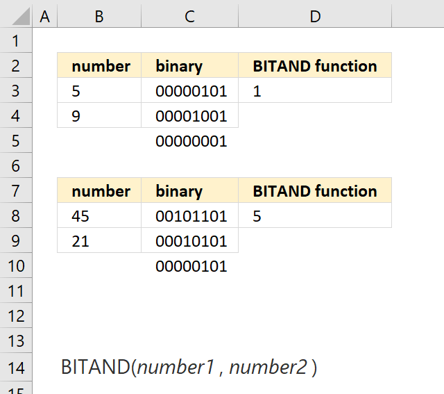
What is the BITAND function?
The BITAND function calculates a bitwise 'AND' of two decimal numbers. Note, it also returns a decimal number.
What is a decimal number?
The decimal system is a positional numeral system that uses 10 as the base, it requires 10 different numerals: 0, 1, 2, 3, 4, 5, 6, 7, 8, and 9. The dot or the decimal point represents decimal fractions which are not whole numbers.
The decimal number 520 has three positions, each with a different weight. It starts with 10^0 on the right and increases by one power on each additional position to the left.
520 = (5*10^2)+(2*10^1)+(0*10^0)
520 = 500 + 20 + 0
What is a bit?
The binary system is a positional numeral system that uses only two digits: 0 and 1. The binary system is important in our society, many devices like computers, digital cameras, mobile phones and modern cars use binary code to store, process and communicate data. The binary numeral system makes it easy to store and transmit data using binary digits or bits.
The following table shows decimal numbers from 0 to 11 and the binary equivalent:
| Decimal | Binary |
| 0 | 0 |
| 1 | 1 |
| 2 | 10 |
| 3 | 11 |
| 4 | 100 |
| 5 | 101 |
| 6 | 110 |
| 7 | 111 |
| 8 | 1000 |
| 9 | 1001 |
| 10 | 1010 |
| 11 | 1011 |
What is bitwise?
Bitwise operations are performed on the binary representation of numbers, where each bit has a value of either 0 or 1. Some common bitwise operations are AND, OR, XOR, NOT and SHIFT. They can be used for masking, toggling, swapping, testing or arithmetic. This article demonstrates AND operations.
What is an AND operation?
The BITAND function performs AND logic bit by bit on the numbers based on their binary representation. AND logic means that the value of each bit position is counted only if both parameter's bits at that position are 1.
The following operations show that AND logic is the same as multiplying binary numbers:
0*0=0
1*0=0
0*1=0
1*1=1
Example, the table below shows bitwise AND logic between two random binary numbers.
| Bit position | 3 | 2 | 1 | 0 |
| Binary value 1 | 1 | 0 | 0 | 1 |
| Binary value 2 | 0 | 1 | 0 | 1 |
| AND result | 0 | 0 | 0 | 1 |
Bit position 0 is the only operation that has 1 in both bits, the remaining bits result in 0 (zero).
Table of Contents
1. BITAND function Syntax
BITAND(number1, number2)
2. BITAND function Arguments
| number1 | Required. The first number. |
| number2 | Required. The second number. |
3. BITAND function example
The image above shows the BITAND function cell D3, it has two arguments number 1 and number2 which are specified in cells B3 and B4.
Formula in cell B3:
The formula in cell B3 performs AND logic for each bit between decimal numbers and returns a decimal number.
4. How is the BITAND function calculated in detail?
Here are the steps to perform bitwise AND logic:
- Convert both decimal numbers to binary.
- Perform bitwise AND logic.
- Convert binary output back to decimal again.
Example 1,
Decimal number 5 is 0000 0101 in binary and decimal number 9 is 0000 1001 in binary.
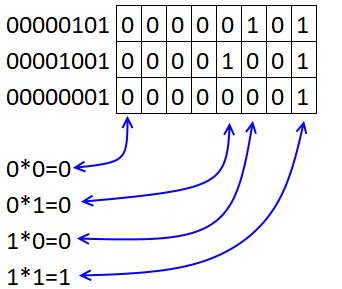
With AND logic bitwise the result is 0000 0001 which is number 1.
Example 2,
Decimal number 45 is 0010 1101 in binary and decimal number 21 is 0001 0101 in binary.
| Bit position | 7 | 6 | 5 | 4 | 3 | 2 | 1 | 0 |
| Binary value 1 | 0 | 0 | 1 | 0 | 1 | 1 | 0 | 1 |
| Binary value 2 | 0 | 0 | 0 | 1 | 0 | 1 | 0 | 1 |
| AND result | 0 | 0 | 0 | 0 | 0 | 1 | 0 | 1 |
The bitwise AND logic results in 0000 0101 which is the decimal number 5.
5. BITAND function not working

The BITAND function returns a #NUM! error if
- argument number is 2^48 = 2.81475E+14 or larger. See row 4 in the image above.
- argument number is negative. See row 3 in the image above.
The BITAND function returns a #VALUE! error if the argument is a letter. See row 5 in the image above.
The BITAND function seems to work with boolean values TRUE and FALSE. See row 6 in the image above.
6. How to perform bitwise AND operations between binary numbers?

The following example demonstrates a formula that lets you calculate bitwise AND logic between two binary numbers, the result is also binary.
Formula:
Explaining formula
Step 1 - Convert binary to decimal
The BIN2DEC function converts a binary number to the decimal number system.
Function syntax: BIN2DEC(number)
BIN2DEC(B3)
becomes
BIN2DEC("00000101")
and returns 5.
Step 2 - Perform bitwise AND operation
The BITAND function calculates a bitwise 'AND' of two numbers.
Function syntax: BITAND(number1, number2)
BITAND(BIN2DEC(B3),BIN2DEC(C3))
becomes
BITAND(5,101)
and returns 5.
Step 3 - Convert result to back to binary
The DEC2BIN function converts a decimal number to a binary number.
Function syntax: DEC2BIN(number, [places])
DEC2BIN(BITAND(BIN2DEC(B3),BIN2DEC(C3)))
becomes
DEC2BIN(5)
and returns "00000101".
Useful resources
BITAND function - Microsoft
Bitwise operation - Wikipedia
5. How to use the BITLSHIFT function
What is the BITLSHIFT function?
The BITLSHIFT function calculates a decimal number whose binary representation is shifted left by a specified number of bits.
What is the binary system?
The binary system is a positional numeral system that uses only two digits: 0 and 1. The binary system is important in our society, many devices like computers, digital cameras, mobile phones and modern cars use binary code to store, process and communicate data. The binary numeral system makes it easy to store and transmit data using binary digits or bits.
The following table shows decimal numbers from 0 to 11 and the binary equivalent:
| Decimal | Binary |
| 0 | 0000 |
| 1 | 0001 |
| 2 | 0010 |
| 3 | 0011 |
| 4 | 0100 |
| 5 | 0101 |
| 6 | 0110 |
| 7 | 0111 |
| 8 | 1000 |
| 9 | 1001 |
| 10 | 1010 |
| 11 | 1011 |
What are bits?
A bit is a binary digit meaning the single digit in a binary number. Binary numbers are often split into four bits, four bits represents decimal numbers from 0 to 15 or hexadecimal numbers from 0 to F. For example, binary number 0010 has four bits.
What is bits shifted left?
Each bit is moved one position to the left, the easiest way to do this is to add a zero on the right side of the binary number.
The result of shifting bits left is the same as multiplying the original value by a power of two. For example, shift decimal value 10 left by one position we get 20 which is 10 times 2. If we shift it left by two positions we get 40 which is 10 * 2 * 2
Decimal value 10 is 1010 in the binary system. Add a zero to the right side and we get 10100 which is 20 in the decimal system.
Why shift bits left?
Bits shifted left can be used for performing arithmetic operations, manipulating bits, or encoding data. However, the BITLSHIFT function works only for positive decimal numbers. It is therefore not possible to change the significant bit when shifting left.
What are significant bits?
The significant bit or sign bit indicates whether a binary number is positive or negative, if the bit is 0 the number is positive, if the bit is 1, the number is negative.
What is a magnitude bit?
The remaining bits are magnitude bits which represents the absolute value of the number. An absolute number is a number without the sign.
Table of Contents
1. BITLSHIFT Function Syntax
BITLSHIFT(number, shift_amount)
2. BITLSHIFT Function Arguments
| number | Required. The number you want to shift. Must be 0 (zero) or greater than 0 (zero). |
| shift_amount | Required. How many zeros you want to add to the right side. This number can be negative as well, |
3. BITLSHIFT function example
The image above demonstrates a formula in cell D3 that shifts bits left based on a decimal number specified in cell B3, the number of positions shifted left is specified in cell C3.
Formula in cell D3:
Example 1,
Cell B3 contains decimal number 5 which is 0101 in the binary system. Add a 0 (zero) to the right side and you get 1010 binary which is number 10 in the decimal system.
Example 2,
Cell B8 contains decimal number 41 which is 0010 1001 in the binary system, cell C8 contains 1 which means that the binary digits are shifted left by one position. Add a 0 (zero) to the right side and you get 0101 0010 in binary which is number 82 in the decimal system.
4. How is the BITLSHIFT function calculated in detail?
The table below shows how bits are shifted left using the BITLSHIFT function by one position.
| Bit position | 3 | 2 | 1 | 0 |
| Binary value 5 | 0 | 1 | 0 | 1 |
| BITLSHIFT result | 1 | 0 | 1 | 0 |
Simply add a 0 (zero) to the right side of the binary number to shift bits one step, this applies to multiple steps as well.
For example, to shift bits three steps left add the same amount of 0's (zeros) to the right side of the binary number, in this example three 0's (zeros).
Decimal number 5 is 0101 in the binary system, shifting bits 3 positions results in this binary number: 0010 1000 which is equal to decimal number 40.
5. BITLSHIFT function not working

The BITLSHIFT function returns a #NUM! error if
- argument number is 2^48 = 2.81475E+14 or larger. See row 4 in the image above.
- argument number is negative. See row 3 in the image above.
- argument number is smaller than 0 (zero).
The BITLSHIFT function returns a #VALUE! error if either of the argument is a letter. See row 5 in the image above.
The BITLSHIFT function seems to work with boolean values TRUE and FALSE. See row 6 in the image above.
6. How to shift bits using binary numbers?

The BITLSHIFT function needs a decimal number to be able to shift the binary representation left and the return the decimal representation of the shifted bits.
The following formula lets you shift binary numbers based on a given number of shifts, the result is also a binary number.
Formula in cell D3:
The formula is limited by the BIN2DEC and DEC2BIN functions, they can only handle decimal numbers from -512 to 511.
The following formula works for larger numbers:
However, this may create a new problem with the sign bit that shows if a binary number is positive or negative.
Explaining formula
Step 1 - Convert binary number to decimal the system
The BIN2DEC function converts a binary number to the decimal number system.
Function syntax: BIN2DEC(number)
BIN2DEC(B3)
becomes
BIN2DEC("00000101")
and returns 5
Step 2 - Shift bits to the left
The BITLSHIFT function calculates a number whose binary representation is shifted left by a specified number of bits.
Function syntax: BITLSHIFT(number, shift_amount)
BITLSHIFT(BIN2DEC(B3),C3)
becomes
BITLSHIFT(5,1)
and returns 10
Step 3 - Convert result to binary
The DEC2BIN function converts a decimal number to a binary number.
Function syntax: DEC2BIN(number, [places])
DEC2BIN(BITLSHIFT(BIN2DEC(B3),C3))
becomes
DEC2BIN(10)
and returns
"1010".
Useful resources
BITLSHIFT function - Microsoft support
Bit shifts - Wikipedia
6. How to use the BITOR function
What is the BITOR function?
The BITOR function performs a bitwise 'OR' of two decimal numbers, it returns a decimal number as well.
What is a decimal number?
The decimal system is a positional numeral system that uses 10 as the base, it requires 10 different numerals: 0, 1, 2, 3, 4, 5, 6, 7, 8, and 9. The dot or the decimal point represents decimal fractions which are not whole numbers.
The decimal number 520 has three positions, each with a different weight. It starts with 10^0 on the right and increases by one power on each additional position to the left.
520 = (5*10^2)+(2*10^1)+(0*10^0)
520 = 500 + 20 + 0
What is a bit?
The binary system is a positional numeral system that uses only two digits: 0 and 1. The binary system is important in our society, many devices like computers, digital cameras, mobile phones and modern cars use binary code to store, process and communicate data. The binary numeral system makes it easy to store and transmit data using binary digits or bits.
The following table shows decimal numbers from 0 to 11 and the binary equivalent:
| Decimal | Binary |
| 0 | 0 |
| 1 | 1 |
| 2 | 10 |
| 3 | 11 |
| 4 | 100 |
| 5 | 101 |
| 6 | 110 |
| 7 | 111 |
| 8 | 1000 |
| 9 | 1001 |
| 10 | 1010 |
| 11 | 1011 |
What is bitwise?
Bitwise operations are performed on the binary representation of numbers, where each bit has a value of either 0 or 1. Some common bitwise operations are AND, OR, XOR, NOT and SHIFT. They can be used for masking, toggling, swapping, testing or arithmetic. This article demonstrates OR operations.
What is an OR operation?
The BITOR function performs OR logic bit by bit on the numbers based on their binary representation. OR logic means that the value of each bit position is counted only if at least one parameter's bits at that position are 1.
The following operations show that OR logic is the same as adding binary numbers:
0+0=0
1+0=1
0+1=0
1+1=1
Example, the table below shows bitwise OR logic between two random binary numbers.
| Bit position | 3 | 2 | 1 | 0 |
| Binary value 1 | 1 | 0 | 0 | 1 |
| Binary value 2 | 0 | 1 | 0 | 1 |
| OR result | 1 | 1 | 0 | 1 |
Bit position 1 is the only operation that has 0 in both bits, the remaining bits result in 1.
Table of Contents
1. BITOR Function Syntax
BITOR(number1, number2)
2. BITOR Function Arguments
| number1 | Required. The first number. |
| number1 | Required. The second number. |
3. BITOR Function example
The image above demonstrates the BITOR function in cell D3, the arguments are in cells B3 and B4 respectively.
Formula in cell D3:
Cells C3 and C4 shows the binary representation of the decimal numbers in cells B3 and B4. The BITOR function in cell D3 returns 13 from the decimal numbers 5 and 9.
The second example is demonstrated in cell D8:
The BITOR function in cell D8 returns 61 from decimal numbers 45 and 21.
The next sections explains how bitwise OR logic works.
4. How is the BITOR function calculated in detail?
Here are the steps to perform bitwise OR logic:
- Convert both decimal numbers to binary.
- Perform bitwise OR logic.
- Convert binary output back to decimal again.
Example 1
Number 5 is 0000 0101 in binary and number 9 is 0000 1001. If at least one bit is 1 the returning digit is 1.
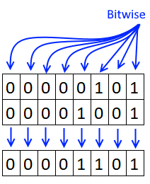
101 + 1101 = 1101. 1101 is the decimal number 13.
Example 2
Number 45 is 0010 1101 in binary and number 21 is 0001 0101. If at least one bit is 1 the returning digit is 1.
| Bit position | 7 | 6 | 5 | 4 | 3 | 2 | 1 | 0 |
| Decimal number 45 | 0 | 0 | 1 | 0 | 1 | 1 | 0 | 1 |
| Decimal number 21 | 0 | 0 | 0 | 1 | 0 | 1 | 0 | 1 |
| OR result | 0 | 0 | 1 | 1 | 1 | 1 | 0 | 1 |
The bitwise OR operation results in 0011 1101 which is decimal number 61.
5. BITOR Function not working

The BITOR function returns a #NUM! error if
- argument number is 2^48 = 2.81475E+14 or larger. See row 4 in the image above.
- argument number is negative. See row 3 in the image above.
The BITOR function returns a #VALUE! error if the argument is a letter. See row 5 in the image above.
The BITAND function seems to work with boolean values TRUE and FALSE. See row 6 in the image above.
6. How to perform bitwise OR operations between binary numbers?

The following formula lets you perform bitwise OR logic based on binary numbers, the result is also a binary number.
Formula:
Cells C3 and C4 shows the decimal representation of the specified binary numbers in cells B3 and B4, cells C3 and C4 are not needed. They are only shown for clarification.
Explaining formula
Step 1 - Convert binary number to decimal the system
The BIN2DEC function converts a binary number to the decimal number system.
Function syntax: BIN2DEC(number)
BIN2DEC(B3)
becomes
BIN2DEC("00000101")
and returns 5
Step 2 - Perform bitwise XOR operation
The BITOR function performs a bitwise 'OR' of two numbers.
Function syntax: BITOR(number1, number2)
BITOR(BIN2DEC(B3),BIN2DEC(C3))
becomes
BITOR(5,9)
and returns 13
Step 3 - Convert result to binary
The DEC2BIN function converts a decimal number to a binary number.
Function syntax: DEC2BIN(number, [places])
DEC2BIN(BITOR(BIN2DEC(B3),BIN2DEC(C3)),8)
beomes
DEC2BIN(13)
and returns
"00001101".
Useful resources
BITOR function - Microsoft support
Bitwise OR - wikipedia
7. How to use the BITRSHIFT function
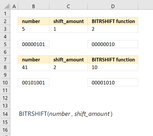
What is the BITRSHIFT function?
The BITRSHIFT function calculates a number based on the decimal system whose binary representation is shifted right by a given number of bits.
What is the binary system?
The binary system is a positional numeral system that uses only two digits: 0 and 1. The binary system is important in our society, many devices like computers, digital cameras, mobile phones and modern cars use binary code to store, process and communicate data. The binary numeral system makes it easy to store and transmit data using binary digits or bits.
The following table shows decimal numbers from 0 to 11 and the binary equivalent:
| Decimal | Binary |
| 0 | 0000 |
| 1 | 0001 |
| 2 | 0010 |
| 3 | 0011 |
| 4 | 0100 |
| 5 | 0101 |
| 6 | 0110 |
| 7 | 0111 |
| 8 | 1000 |
| 9 | 1001 |
| 10 | 1010 |
| 11 | 1011 |
What are bits?
A bit is a binary digit meaning the single digit in a binary number. Binary numbers are often split into four bits, four bits represents decimal numbers from 0 to 15 or hexadecimal numbers from 0 to F. For example, binary number 0010 has four bits.
What is bits shifted right?
Each bit is moved one position to the right, the easiest way to do this is to add a zero on the left side of the binary number and remove the last digit on the right side to shift bits one position.
Why shift bits right?
Bits shifted left can be used for performing arithmetic operations, manipulating bits, or encoding data. The BITRSHIFT function works only for positive numbers in the decimal system, there is no risk of changing the significant bit when shifting right.
What is the significant bit?
The significant bit or sign bit indicates whether a binary number is positive or negative, if the bit is 0 the number is positive, if the bit is 1, the number is negative.
What is a magnitude bit?
The remaining bits are magnitude bits which represents the absolute value of the number. An absolute number is a number without the sign.
Table of Contents
1. BITRSHIFT Function Syntax
BITRSHIFT(number, shift_amount)
2. BITRSHIFT Function Arguments
| number | Required. The number you want to shift. Must be 0 (zero) or greater than 0 (zero). |
| shift_amount | Required. How many zeros you want to add to the right side. This number can be negative as well, |
3. BITRSHIFT function example
The image above demonstrates a formula in cell D3 that shifts bits right based on a decimal number specified in cell B3, the number of positions shifted right is specified in cell C3.
Formula in cell D3:
Example 1,
Cell B3 contains decimal number 5 which is 0101 in the binary system. Add a 0 (zero) to the left side and remove the last bit on the right side and you get 0010 binary which is number 2 in the decimal system.
Example 2,
Cell B8 contains decimal number 41 which is 0010 1001 in the binary system, cell C8 contains 2 which means that the binary digits are shifted right by two positions. Add two 0's (zeros) to the left side and remove two bits on the right side and you get 0000 1010 in binary which is number 10 in the decimal system.
4. How is the BITRSHIFT function calculated in detail?
The table below shows how bits are shifted right using the BITRSHIFT function by one position.
| Bit position | 3 | 2 | 1 | 0 |
| Binary value 5 | 0 | 1 | 0 | 1 |
| BITRSHIFT result | 0 | 0 | 1 | 0 |
To shift bits one position to the right add a 0 (zero) to the left side of the binary number and remove the last bit on the right side.
Example 2, to shift bits two steps right add the same amount of 0's (zeros) to the left side of the binary number, in this example two 0's (zeros).
Decimal number 5 is 0101 in the binary system, shifting bits 2 positions results in this binary number: 0001 which is equal to decimal number 1.
5. BITRSHIFT function not working

The BITRSHIFT function returns a #NUM! error if
- argument number is 2^48 = 2.81475E+14 or larger. See row 3 in the image above.
- argument number is negative.
- argument number is smaller than 0 (zero).
- argument shift_amount is larger than 53
The BITRSHIFT function returns a #VALUE! error if either of the argument is a letter. See row 5 in the image above.
The BITRSHIFT function seems to work with boolean values TRUE and FALSE. See row 6 in the image above.
6. How to shift bits with binary numbers?

The BITRSHIFT function needs a decimal number to be able to shift the binary representation right and the return the decimal representation of the shifted bits.
The following formula lets you shift binary numbers based on a given number of shifts, the result is also a binary number.
Formula in cell D3:
The formula is limited by the BIN2DEC and DEC2BIN functions, they can only handle decimal numbers from -512 to 511.
The following formula works for larger numbers:
However, this may create a new problem with the sign bit that shows if a binary number is positive or negative.
Explaining formula
Step 1 - Convert binary number to decimal the system
The BIN2DEC function converts a binary number to the decimal number system.
Function syntax: BIN2DEC(number)
BIN2DEC(B3)
becomes
BIN2DEC("00000101")
and returns 5
Step 2 - Shift bits to the right
The BITRSHIFT function calculates the number where the binary equivalent is shifted right by a specified number of bits and then converted back to a number.
Function syntax: BITRSHIFT(number, shift_amount)
BITRSHIFT(BIN2DEC(B3),C3)
becomes
BITRSHIFT(5,1)
and returns 2
Step 3 - Convert result to binary
The DEC2BIN function converts a decimal number to a binary number.
Function syntax: DEC2BIN(number, [places])
DEC2BIN(BITRSHIFT(BIN2DEC(B3),C3))
becomes
DEC2BIN(2)
and returns
"0010".
Useful resources
BITRSHIFT function - Microsoft support
Bit shifts - Wikipedia
8. How to use the BITXOR function
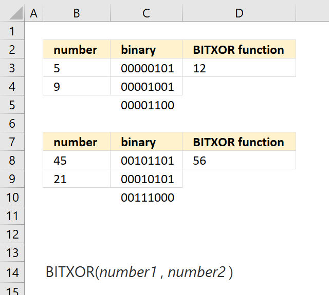
What is the BITXOR function?
The BITXOR function calculates a decimal number that is a result of a bitwise comparison "XOR" of two decimal numbers, XOR stands for Exclusive OR.
What is a decimal number?
The decimal system is a positional numeral system that uses 10 as the base, it requires 10 different numerals: 0, 1, 2, 3, 4, 5, 6, 7, 8, and 9. The dot or the decimal point represents decimal fractions which are not whole numbers.
The decimal number 520 has three positions, each with a different weight. It starts with 10^0 on the right and increases by one power on each additional position to the left.
520 = (5*10^2)+(2*10^1)+(0*10^0)
520 = 500 + 20 + 0
What is a bit?
The binary system is a positional numeral system that uses only two digits: 0 and 1. The binary system is important in our society, many devices like computers, digital cameras, mobile phones and modern cars use binary code to store, process and communicate data. The binary numeral system makes it easy to store and transmit data using binary digits or bits.
The following table shows decimal numbers from 0 to 11 and the binary equivalent:
| Decimal | Binary |
| 0 | 0000 |
| 1 | 0001 |
| 2 | 0010 |
| 3 | 0011 |
| 4 | 0100 |
| 5 | 0101 |
| 6 | 0110 |
| 7 | 0111 |
| 8 | 1000 |
| 9 | 1001 |
| 10 | 1010 |
| 11 | 1011 |
What is bitwise?
Bitwise operations are performed on the binary representation of numbers, where each bit has a value of either 0 or 1. Some common bitwise operations are AND, OR, XOR, NOT and SHIFT. They can be used for masking, toggling, swapping, testing or arithmetic. This article demonstrates XOR operations.
What is an XOR operation?
The BITXOR function performs XOR logic bit by bit on the numbers based on their binary representation. XOR is an abbreviation for "Exclusive OR" meaning if both digits at each position are not equal, 1 is returned for that position. If they are equal 0 (zero) is returned.
The following operations show how XOR logic work:
0+0=0
1+0=1
0+1=1
1+1=0
Example, the table below shows bitwise XOR logic between two random binary numbers.
| Bit position | 3 | 2 | 1 | 0 |
| Binary value 1 | 1 | 0 | 0 | 1 |
| Binary value 2 | 0 | 1 | 0 | 1 |
| XOR result | 1 | 1 | 0 | 0 |
Table of Contents
1. BITXOR Function Syntax
BITXOR(number1, number2)
2. BITXOR Function Arguments
| number1 | Required. A number greater than 0 (zero). |
| number2 | Required. A number greater than 0 (zero). |
3. BITXOR Function example
The image above demonstrates a formula in cell D3 that performs exclusive OR between two decimal numbers specified in cells B3 and B4. The decimal numbers are automatically converted in to binary digits and then the BITXOR function performs an exclusive OR operation. Lastly, the binary result is then converted back in to a decimal number.
Formula in cell D3:
The image above shows numbers 5 and 9 in cells B3 and B4 respectively. The BITXOR function converts the decimal numbers to binary numbers 0000 0101 and 0000 1001, the exclusive OR is 0000 1100 which represents 12 in the decimal system shown in cell D3.
4. How is the BITXOR function calculated in detail?
Here are the steps to perform bitwise XOR logic:
- Convert both decimal numbers to binary.
- Perform bitwise XOR logic, here are the rules:
0+0=0
1+0=1
0+1=1
1+1=0 - Convert binary output back to decimal again.
Example
5 is 00000101 binary and 9 is 00001001. See picture below on how to do a bitwise "XOR".
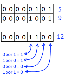
5. BITXOR function not working

The BITXOR function returns a #NUM! error if
- argument number is 2^48 = 2.81475E+14 or larger. See row 4 in the image above.
- argument number is negative. See row 3 in the image above.
The BITOR function returns a #VALUE! error if the argument is a letter. See row 5 in the image above.
The BITAND function seems to work with boolean values TRUE and FALSE. See row 6 in the image above.
6. How to perform bitwise XOR operations between binary numbers?

The following formula lets you perform bitwise XOR logic based on binary numbers, the result is also a binary number.
Formula:
Cells C3 and C4 shows the decimal representation of the specified binary numbers in cells B3 and B4, cells C3 and C4 are not needed. They are only shown for clarification.
Explaining formula
Step 1 - Convert binary number to decimal the system
The BIN2DEC function converts a binary number to the decimal number system.
Function syntax: BIN2DEC(number)
BIN2DEC(B3)
becomes
BIN2DEC("00000101")
and returns 5
Step 2 - Perform bitwise OR operation
The BITXOR function calculates a decimal number that is a result of a bitwise comparison "XOR" of two numbers.
Function syntax: BITXOR(number1, number2)
BITXOR(BIN2DEC(B3),BIN2DEC(C3))
becomes
BITXOR(5,9)
and returns 12
Step 3 - Convert result to binary
The DEC2BIN function converts a decimal number to a binary number.
Function syntax: DEC2BIN(number, [places])
DEC2BIN(BITXOR(BIN2DEC(B3),BIN2DEC(C3)),8)
beomes
DEC2BIN(12)
and returns
"00001100".
Useful resources
BITXOR function - Microsoft support
Bitwise XOR - wikipedia
9. How to use the COMPLEX function
What is the COMPLEX function?
The COMPLEX function returns a complex number in the general form (also known as the rectangular form) based on a real and imaginary number.
What is a complex number?
A complex number can be written in this form x+yi, it contains a real and imaginary part. Complex numbers extend the real numbers by allowing solutions to equations that have no real solutions.
Complex numbers can be represented as points or vectors on a plane called the complex plane, where the horizontal axis is the real axis and the vertical axis is the imaginary axis, see the image above. The complex plane allows a geometric interpretation of complex numbers and their operations.
Table of Contents
1. COMPLEX Function Syntax
COMPLEX(real_num, i_num, [suffix])
2. COMPLEX Function Arguments
| real_num | Required. The real coefficient of the complex number. |
| i_num | Required. The imaginary coefficient of the complex number. |
| [suffix] | Optional. This argument lets you choose the suffix of the imaginary component. The default value is "i". |
The letter j is used in electrical engineering to distinguish between the imaginary value and the electric current.
3. COMPLEX Function example
The COMPLEX function is useful when you want to create a complex number with given real and imaginary coefficients. A complex number is a number that has two parts: a real part and an imaginary part. The real part is a number that you are familiar with, such as 2, -5, or 0.5. The imaginary part is a number that is multiplied by a special symbol called i, which stands for the square root of -1.
The COMPLEX function converts real and imaginary coefficients into a complex number of the form x + yi or x + yj, where x represents the real part and y represents the imaginary part.
The COMPLEX function returns a text result, not a numeric result. You can not perform arithmetic operations on the result directly. However, Excel has other functions that work with complex numbers, check out the Engineering category for more imaginary functions.
Formula in cell E3:
Cell B3 contains the real coefficient of the complex number, x in the diagram. Cell C3 contains the imaginary coefficient of the complex number, y in the diagram shown above.
Cell E3 calculates the complex number based on the real and imaginary coefficients specified in cells B3 and C3 respectively.
3.1 Explaining formula
Step 1 - Populate arguments
COMPLEX(real_num, i_num, [suffix])
becomes
COMPLEX(B3,C3)
Step 2 - Evaluate COMPLEX function
COMPLEX(B3,C3)
becomes
COMPLEX(2,3)
and returns
"2+3i".
The COMPLEX function returns complex numbers in general form.
3.2 What is the general form of complex numbers?
The general form of complex numbers is a + bi, where a and b are real numbers and i is the imaginary unit that satisfies i^2 = -1. The real part of a complex number is a, and the imaginary part is b.
3.3 Describe different forms of complex numbers?
| Form | Description |
| General or rectangular | Z = a +bi. Use this form when you want to perform arithmetic operations such as addition, subtraction, multiplication, and division of complex numbers. It also shows the real and imaginary parts of a complex number clearly. |
| Polar | Z = r(cos θ + i sin θ) This form is useful for finding the roots, powers, and logarithms of complex numbers. It also shows the geometric interpretation of a complex number as a point on the complex plane with a certain distance and direction from the origin. |
| Exponential | Z = re^(iθ) Use this form when you want to simplify calculations involving trigonometric functions and exponential functions of complex numbers. It also shows the connection between complex numbers and periodic phenomena such as waves and oscillations. |
| Standard basis form | Example, 2-3i = 2*1 + (-3)*i This form is useful for performing linear algebra operations such as scalar multiplication, vector addition, dot product, and cross product of complex numbers. It also shows the algebraic structure of complex numbers as a two-dimensional vector space. |
The general form and the polar form of complex numbers are equivalent and can be converted from one to another using trigonometry and algebra.
3.4 Why is i equal to the square root of -1?
The symbol i is defined as the square root of -1 because there is no real number that satisfies this equation. If we try to find a real number x such that x^2 = -1, we get a contradiction.
For example, if x is positive, then x^2 is also positive, so it cannot be equal to -1.
If x is negative, then x^2 is also positive, for the same reason.
If x is zero, then x^2 is also zero, which is not equal to -1. So there is no real solution to x^2 = -1.
However, mathematicians wanted to extend the real numbers to include a solution to this equation, so they invented a new symbol i (iota) and defined it as the square root of -1. This means that i^2 = -1 by definition. This also means that i is not a real number, but an imaginary number.
We can create complex numbers, by using i, which are numbers that have both a real part and an imaginary part. Complex numbers are useful because they allow us to solve equations that have no real solutions, such as x^2 + 1 = 0. Using i, we can find two solutions: x = i and x = -i. This is because i^2 = -1 and (-i)^2 = -1.
4. COMPLEX Function error
The COMPLEX function returns #VALUE error if the two first arguments are not numbers.
The COMPLEX function also returns a #VALUE if the suffix is not "i", "j" or omitted.
Useful resources
COMPLEX function - Microsoft
Intro to complex numbers
An Introduction to Complex Numbers
10. How to use the CONVERT function
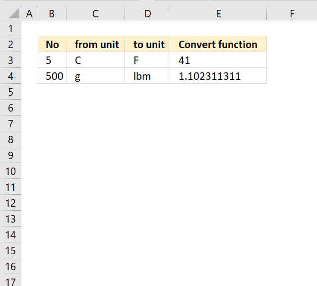
The CONVERT function converts a number from one measurement system to another. It lets you perform conversions in these categories: weight and mass, distances, time, pressure, force, energy, magnetism, temperature, volume, area, speed, and prefixes.
Table of Contents
1. CONVERT Function Syntax
CONVERT(number, from_unit, to_unit)
2. CONVERT Function Arguments
| number | Required. The number you want to convert from. |
| from_unit | Required. The unit you want to convert from. |
| to_unit | Required. The unit you want to convert to. |
| Weight and mass | From_unit or to_unit |
|---|---|
| Gram | "g" |
| Slug | "sg" |
| Pound mass (avoirdupois) | "lbm" |
| U (atomic mass unit) | "u" |
| Ounce mass (avoirdupois) | "ozm" |
| Grain | "grain" |
| U.S. (short) hundredweight | "cwt" or "shweight" |
| Imperial hundredweight | "uk_cwt" or "lcwt" ("hweight") |
| Stone | "stone" |
| Ton | "ton" |
| Imperial ton | "uk_ton" or "LTON" ("brton") |
| Distance | From_unit or to_unit |
|---|---|
| Meter | "m" |
| Statute mile | "mi" |
| Nautical mile | "Nmi" |
| Inch | "in" |
| Foot | "ft" |
| Yard | "yd" |
| Angstrom | "ang" |
| Ell | "ell" |
| Light-year | "ly" |
| Parsec | "parsec" or "pc" |
| Pica (1/72 inch) | "Picapt" or "Pica" |
| Pica (1/6 inch) | "pica" |
| U.S survey mile (statute mile) | "survey_mi" |
| Time | From_unit or to_unit |
|---|---|
| Year | "yr" |
| Day | "day" or "d" |
| Hour | "hr" |
| Minute | "mn" or "min" |
| Second | "sec" or "s" |
| Pressure | From_unit or to_unit |
|---|---|
| Pascal | "Pa" (or "p") |
| Atmosphere | "atm" (or "at") |
| mm of Mercury | "mmHg" |
| PSI | "psi" |
| Torr | "Torr" |
| Force | From_unit or to_unit |
|---|---|
| Newton | "N" |
| Dyne | "dyn" (or "dy") |
| Pound force | "lbf" |
| Pond | "pond" |
| Energy | From_unit or to_unit |
|---|---|
| Joule | "J" |
| Erg | "e" |
| Thermodynamic calorie | "c" |
| IT calorie | "cal" |
| Electron volt | "eV" (or "ev") |
| Horsepower-hour | "HPh" (or "hh") |
| Watt-hour | "Wh" (or "wh") |
| Foot-pound | "flb" |
| BTU | "BTU" (or "btu") |
| Power | From_unit or to_unit |
|---|---|
| Horsepower | "HP" (or "h") |
| Pferdestärke | "PS" |
| Watt | "W" (or "w") |
| Magnetism | From_unit or to_unit |
|---|---|
| Tesla | "T" |
| Gauss | "ga" |
| Temperature | From_unit or to_unit |
|---|---|
| Degree Celsius | "C" (or "cel") |
| Degree Fahrenheit | "F" (or "fah") |
| Kelvin | "K" (or "kel") |
| Degrees Rankine | "Rank" |
| Degrees Réaumur | "Reau" |
| Volume (or l iquid measure ) | From_unit or to_unit |
|---|---|
| Teaspoon | "tsp" |
| Modern teaspoon | "tspm" |
| Tablespoon | "tbs" |
| Fluid ounce | "oz" |
| Cup | "cup" |
| U.S. pint | "pt" (or "us_pt") |
| U.K. pint | "uk_pt" |
| Quart | "qt" |
| Imperial quart (U.K.) | "uk_qt" |
| Gallon | "gal" |
| Imperial gallon (U.K.) | "uk_gal" |
| Liter | "l" or "L" ("lt") |
| Cubic angstrom | "ang3" or "ang^3" |
| U.S. oil barrel | "barrel" |
| U.S. bushel | "bushel" |
| Cubic feet | "ft3" or "ft^3" |
| Cubic inch | "in3" or "in^3" |
| Cubic light-year | "ly3" or "ly^3" |
| Cubic meter | "m3" or "m^3" |
| Cubic Mile | "mi3" or "mi^3" |
| Cubic yard | "yd3" or "yd^3" |
| Cubic nautical mile | "Nmi3" or "Nmi^3" |
| Cubic Pica | "Picapt3", "Picapt^3", "Pica3" or "Pica^3" |
| Gross Registered Ton | "GRT" ("regton") |
| Measurement ton (freight ton) | "MTON" |
| Area | From_unit or to_unit |
|---|---|
| International acre | "uk_acre" |
| U.S. survey/statute acre | "us_acre" |
| Square angstrom | "ang2" or “ang^2" |
| Are | "ar" |
| Square feet | "ft2" or "ft^2" |
| Hectare | "ha" |
| Square inches | "in2" or "in^2" |
| Square light-year | "ly2" or "ly^2" |
| Square meters | "m2" or "m^2" |
| Morgen | "Morgen" |
| Square miles | "mi2" or "mi^2" |
| Square nautical miles | "Nmi2" or "Nmi^2" |
| Square Pica | "Picapt2", "Pica2", "Pica^2" or "Picapt^2" |
| Square yards | "yd2" or "yd^2" |
| Information | From_unit or to_unit |
|---|---|
| Bit | "bit" |
| Byte | "byte" |
| Speed | From_unit or to_unit |
|---|---|
| Admiralty knot | "admkn" |
| Knot | "kn" |
| Meters per hour | "m/h" or "m/hr" |
| Meters per second | "m/s" or "m/sec" |
| Miles per hour | "mph" |
| Prefix | Multiplier | Abbreviation |
|---|---|---|
| yotta | 1E+24 | "Y" |
| zetta | 1E+21 | "Z" |
| exa | 1E+18 | "E" |
| peta | 1E+15 | "P" |
| tera | 1000000000000 | "T" |
| giga | 1000000000 | "G" |
| mega | 1000000 | "M" |
| kilo | 1000 | "k" |
| hecto | 100 | "h" |
| dekao | 10 | "da" or "e" |
| deci | 0.1 | "d" |
| centi | 0.01 | "c" |
| milli | 0.001 | "m" |
| micro | 0.000001 | "u" |
| nano | 0.000000001 | "n" |
| pico | 0.000000000001 | "p" |
| femto | 0.000000000000001 | "f" |
| atto | 1E-18 | "a" |
| zepto | 1E-21 | "z" |
| yocto | 1E-24 | "y" |
| Binary Prefix | Prefix Value | Abbreviation | Derived from |
|---|---|---|---|
| yobi | 2^80 = 1 208 925 819 614 629 174 706 176 | "Yi" | yotta |
| zebi | 2^70 = 1 180 591 620 717 411 303 424 | "Zi" | zetta |
| exbi | 2^60 = 1 152 921 504 606 846 976 | "Ei" | exa |
| pebi | 2^50 = 1 125 899 906 842 624 | "Pi" | peta |
| tebi | 2^40 = 1 099 511 627 776 | "Ti" | tera |
| gibi | 2^30 = 1 073 741 824 | "Gi" | giga |
| mebi | 2^20 = 1 048 576 | "Mi" | mega |
| kibi | 2^10 = 1024 | "ki" | kilo |
3. CONVERT Function example
Formula in cell E3:
The CONVERT function converts from Celsius to Fahrenheit in cell E3.
4. CONVERT Function error

The CONVERT function returns a #N/A error if the unit doesn't exist.
Unit names and prefixes are case-sensitive.
Can the CONVERT Function convert from decimal to binary/hexadecimal/octal?
No, there are dedicated functions for these types of conversions.
DEC2BIN function | DEC2HEX function | DEC2OCT function
Can the CONVERT Function convert from binary to decimal/hexadecimal/octal?
No, there are dedicated functions for these types of conversions.
BIN2DEC function | BIN2HEX function | BIN2OCT function
Can the CONVERT Function convert from hexadecimal to decimal/binary/octal?
No, there are dedicated functions for these types of conversions.
HEX2BIN function | HEX2DEC function | HEX2OCT function
5. Unit conversion tool

I built a unit conversion tool, below is a link the file. It lets you quickly convert a number from a given unit to another given unit using drop down lists. It is a quick and easy way for unit conversions in Excel.
5.1 Here is how the unit conversion tool works

The image above shows the unit conversion tool, it has three cells B3,C3, and D3 containing different drop down lists. The drop down lists in cells C3 and D3 are populated based on the selected category in cell B3.
The drop down list in cell B3 contains these categories: Area, Distance, Energy, Force, Information, Power, Pressure, Speed, Temperature, Time, Volume, Weight and mass.
Cell B6 lets you specify the number you want to convert, cell C3 specifies the unit and cell D3 specifies which unit you want to convert to. The result is calculated in cell C6, the image above demonstrates how to convert from 1 feet to meter. The result is 0.3048 meter. The chosen category in cell B3 is "Distance", cell C3 contains "ft" and cell D3 contains "m".
5.2 Here is how I built it
I copied and pasted all arguments to one table. I copied the header name for each category to column H.

I removed all double quotes and removed everything after "or". For example, one unit was specified like this: "day" or "d". After removing double quotes and "or ...": day

I then created a formula that extracts unique distinct category names from cell range H3:H128.
Excel 365 formula in cell N3:
The formula also sorts the category names from A to Z, the result is a dynamic array that spills its values to cells below automatically.

I inserted a drop down list to cell B3.
- Select cell B3.
- Go to tab "Data" on the ribbon.
- Press with left mouse button on the "Data Validation" button.

- Press with left mouse button on the "Data Validation...", a dialog box appears.

- Select "List" below "Allow:".
- Select cell N3 below "Source:", make sure it ends with a hashtag. This makes sure that every value from the Excel 365 dynamic array is included.
- Press with left mouse button on the "OK" button.

I then created a formula that extracts units based on the selected value in cell B3.
Excel 365 dynamic array formula in cell O3:
This formula extracts the corresponding units to the selected category and sorts them from A to Z.

I then inserted drop down lists to cells C3 and D3, see the steps above on how to configure these drop down lists. The source cells are both O3#.
The last formula is the CONVERT function, it uses the specified values in cells B6, C3, and D3 to perform the conversion.
Formula in cell C6:
Useful resources
CONVERT Function - Microsoft
Unit converter
Unit conversion
Date and Time Functions – N to Z 18 Mar 2024 2:10 AM (2 years ago)
Table of Contents
- How to use the NETWORKDAYS function
- How to use the NETWORKDAYS.INTL function
- How to use the NOW function
- How to use the SECOND function
- How to use the TIME function
- How to use the TIMEVALUE function
- How to use the TODAY function
- How to use the WEEKDAY function
- How to use the WEEKNUM function
- How to use the WORKDAY function
- How to use the YEAR function
- How to use the YEARFRAC function
1. How to use the NETWORKDAYS function
The NETWORKDAYS function returns the number of working days between two dates, excluding weekends. It also allows you to ignore a list of holiday dates that you can specify.
Formula in cell D3:
What is the difference between the NETWORKDAYS.INTL function and the NETWORKDAYS function?
The NETWORKDAYS.INTL function lets you use custom weekend parameters. Actually they don't have to be a week end day, it can be a weekday also. This makes it really versatile for all sorts of calculations like how many mondays are there between a given start and end date.
Related functions
| Excel Function | Description |
|---|---|
| NETWORKDAYS.INTL(start_date, end_date, weekend) | Returns the number of workdays between two dates, excluding custom weekend parameters |
| NETWORKDAYS(start_date, end_date) | Returns the number of workdays between two dates, excluding weekends |
| WORKDAY(start_date, days) | Returns a date adjusted by a number of workdays, excluding weekends |
| DATEDIF(start_date, end_date, unit) | Calculates the time between two dates in specified units like years, months, days |
| DAYS(end_date, start_date) | Returns the number of days between two specified dates |
Table of Contents
1. NETWORKDAYS Function Syntax
NETWORKDAYS(start_date, end_date, [holidays])
2. NETWORKDAYS Function Arguments
| start_date | Required. The start date you want to use in the function. |
| end_date | Required. The end date you want to use. |
| [holidays] | Optional. Excludes this list of dates from being counted. |
3. NETWORKDAYS Function example

The formula in cell K6 counts weekdays (Monday to Friday) between two dates.
Formula in cell K6:
3.1 Explaining formula
Step 1 - NETWORKDAYS function
The NETWORKDAYS function returns the number of working days between two dates, excluding weekends. It also allows you to ignore a list of holiday dates that you can specify.
NETWORKDAYS(start_date, end_date, [holidays])
Step 2 - Populate arguments
The NETWORKDAYS function has three arguments, the third is optional.
start_date - K3
end_date - K4
[holidays] - Not used here
Step 3 - Evaluate NETWORKDAYS function
NETWORKDAYS(K3, K4)
becomes
NETWORKDAYS(44631, 44648)
and returns 12.
4. Create a list of weekdays only

This example demonstrates how to extract a list of weekdays (Monday to Friday) or networking days. The formula in cell J7 uses the two dates specified in cells K3 and K4 to create a list of weekdays.
Excel 365 formula:
Explaining formula
This formula is a dynamic array formula and works only in Excel 365, it is entered as a regular formula
Step 1 - Calculate days between dates and add one
The minus and plus signs let you perform arithmetic operations in an Excel formula.
K4-K3+1
becomes
44648-44631+1
equals 18.
Step 2 - Create a sequence of numbers from 0 (zero) to 18
The SEQUENCE function creates a list of sequential numbers to a cell range or array. It is located in the Math and trigonometry category and is only available to Excel 365 subscribers.
SEQUENCE(rows, [columns], [start], [step])
SEQUENCE(K4-K3+1,,0)
becomes
SEQUENCE(18,,0)
and returns
{0; 1; 2; 3; 4; 5; 6; 7; 8; 9; 10; 11; 12; 13; 14; 15; 16; 17}.
Step 3 - Add start date to sequence of numbers
SEQUENCE(K4-K3+1,,0)+K3
becomes
{0; 1; 2; 3; 4; 5; 6; 7; 8; 9; 10; 11; 12; 13; 14; 15; 16; 17} + 44631
and returns
{44631; 44632; 44633; 44634; 44635; 44636; 44637; 44638; 44639; 44640; 44641; 44642; 44643; 44644; 44645; 44646; 44647; 44648}.
Step 4 - Calculate WEEKDAY number
WEEKDAY(SEQUENCE(K4-K3+1,,0)+K3,1)
becomes
WEEKDAY({44631; 44632; 44633; 44634; 44635; 44636; 44637; 44638; 44639; 44640; 44641; 44642; 44643; 44644; 44645; 44646; 44647; 44648},1)
and returns
{6; 7; 1; 2; 3; 4; 5; 6; 7; 1; 2; 3; 4; 5; 6; 7; 1; 2}.
Step 5 - Check if weekday number is smaller than 7
Seven is the last weekday in a week and it represents Saturday if the second argument is one. The smaller than character lets you compare values, the result is a boolean value TRUE or FALSE.
WEEKDAY(SEQUENCE(K4-K3+1,,0)+K3,1)<7
becomes
{6; 7; 1; 2; 3; 4; 5; 6; 7; 1; 2; 3; 4; 5; 6; 7; 1; 2}<7
and returns
{TRUE; FALSE; TRUE; TRUE; TRUE; TRUE; TRUE; TRUE; FALSE; TRUE; TRUE; TRUE; TRUE; TRUE; TRUE; FALSE; TRUE; TRUE}.
Step 6 - Check if weekday numbers are larger than one
One represents Sunday and we want to identify dates thare equal to Monday to Friday, in other words, networkingdays.
WEEKDAY(SEQUENCE(K4-K3+1,,0)+K3,1)>1
becomes
{6; 7; 1; 2; 3; 4; 5; 6; 7; 1; 2; 3; 4; 5; 6; 7; 1; 2}>1
and returns
{TRUE; TRUE; FALSE; TRUE; TRUE; TRUE; TRUE; TRUE; TRUE; FALSE; TRUE; TRUE; TRUE; TRUE; TRUE; TRUE; FALSE; TRUE}.
Step 7 - Multiply arrays
Both values on the same position in the arrays must return TRUE meaning we need to perform AND-logic. The asterisk lets us multiply values in an Excel formula.
TRUE * TRUE = 1
TRUE * FALSE = 0 (zero)
FALSE * FALSE = 0 (zero)
Boolean values have numerical equivalents, TRUE is equal to 1 and FALSE is equal to 0 (zero).
(WEEKDAY(SEQUENCE(K4-K3+1,,0)+K3,1)<7)*(WEEKDAY(SEQUENCE(K4-K3+1,,0)+K3,1)>1)
becomes
{TRUE; FALSE; TRUE; TRUE; TRUE; TRUE; TRUE; TRUE; FALSE; TRUE; TRUE; TRUE; TRUE; TRUE; TRUE; FALSE; TRUE; TRUE} * {TRUE; TRUE; FALSE; TRUE; TRUE; TRUE; TRUE; TRUE; TRUE; FALSE; TRUE; TRUE; TRUE; TRUE; TRUE; TRUE; FALSE; TRUE}
and returns
{1; 0; 0; 1; 1; 1; 1; 1; 0; 0; 1; 1; 1; 1; 1; 0; 0; 1}.
Step 8 - Filter dates based on conditions
The FILTER function is a new function available to Excel 365 subscribers. It lets you extract values based on a condition or criteria.
FILTER(array, include, [if_empty])
FILTER(SEQUENCE(K4-K3+1,,0)+K3,(WEEKDAY(SEQUENCE(K4-K3+1,,0)+K3,1)<7)*(WEEKDAY(SEQUENCE(K4-K3+1,,0)+K3,1)>1))
becomes
FILTER({44631; 44632; 44633; 44634; 44635; 44636; 44637; 44638; 44639; 44640; 44641; 44642; 44643; 44644; 44645; 44646; 44647; 44648},{1; 0; 0; 1; 1; 1; 1; 1; 0; 0; 1; 1; 1; 1; 1; 0; 0; 1})
and returns
{44631; 44634; 44635; 44636; 44637; 44638; 44641; 44642; 44643; 44644; 44645; 44648}.
Step 9 - Shorten formula
The LET function allows you to name intermediate calculation results which can shorten formulas considerably and improve performance.
LET(name1, name_value1, calculation_or_name2, [name_value2, calculation_or_name3...])
x - SEQUENCE(K4-K3+1, , 0)+K3
y - WEEKDAY(x, 1)
LET(x, SEQUENCE(K4-K3+1, , 0)+K3, y, WEEKDAY(x, 1), COUNT(FILTER(x, (y<7)*(y>1))))
5. Count weekdays in a month

Formula in cell K6:
Explaining formula
Steps 1 to 3 calculate the first date of the specified month in cell K3. Steps 4 to 6 calculate the last date in the specified month.
Step 1 - Calculate year based on date
The YEAR function returns a number representing the year from a given date.
YEAR(date)
YEAR(K3)
becomes
YEAR(44631)
and returns 2022.
Step 2 - Calculate month based on date
The MONTH function returns a number representing the month from a given date.
MONTH(date)
MONTH(K3)
becomes
MONTH(44631)
and returns 3.
Step 3 - Calculate first date based on year and month
The DATE function returns an Excel date based on a year, month, and day number.
DATE(year, month, day)
DATE(YEAR(K3), MONTH(K3), 1)
becomes
DATE(2022, 3, 1)
and returns 44621. (3/1/2022)
Step 4 - Calculate year based on the date
YEAR(K3)
becomes
YEAR(44631)
and returns 2022.
Step 5 - Calculate year based on month
MONTH(K3)+1
becomes
MONTH(44631)+1
and returns 4.
Step 6 - Calculate the last date based on year and month
DATE(YEAR(K3),MONTH(K3)+1,1)-1
becomes
DATE(2022, 4, 1)-1
becomes
44652-1
and returns 44651. (3/31/2022)
Step 7 - Calculate the number of days between two dates
NETWORKDAYS(DATE(YEAR(K3),MONTH(K3),1),DATE(YEAR(K3),MONTH(K3)+1,1)-1)
becomes
NETWORKDAYS(44621, 44651)
and returns 23.
6. NETWORKDAYS Function - holidays
Excel contains a great function that easily counts the number of workdays between two dates, it even allows you to specify holidays that are not counted.
Formula in cell C4:
The image above shows two dates in cell range B5:B6 that acts as holidays in this example.
Formula in cell C8:
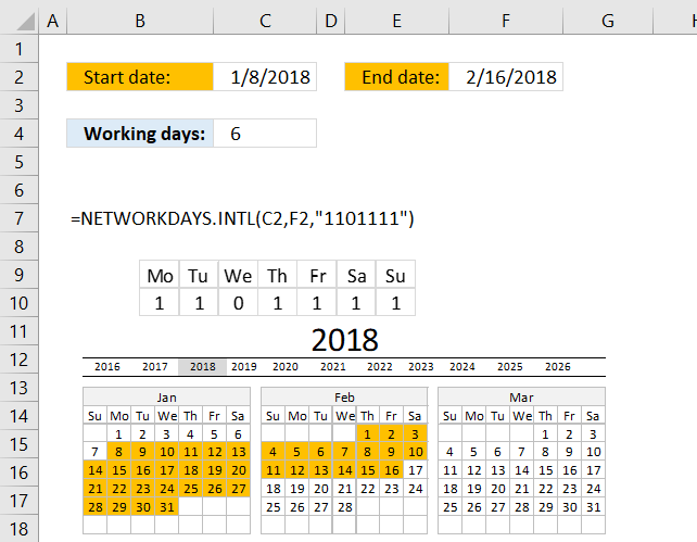
NETWORKDAYS.INTL function is available for Excel 2010 and later versions, it allows you to use custom weekends meaning if you want only Sundays to be weekend you can do that.
The string "1101111" means that all days except Wednesdays are weekends (isn't that great?) in the formula above, see row 9 and 10 above.
2. How to use the NETWORKDAYS.INTL function
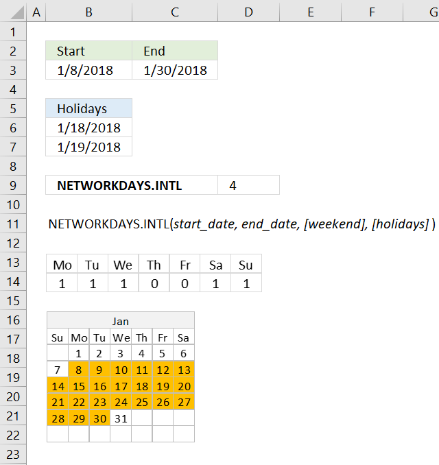
What is the NETWORKDAYS.INTL function?
The NETWORKDAYS.INTL function calculate the number of working days between two dates, excluding weekends. It also allows you to ignore a list of holiday dates that you can specify. You may specify which days are weekend days.
What is the difference between the NETWORKDAYS.INTL function and the NETWORKDAYS function?
The NETWORKDAYS.INTL function lets you use custom weekend parameters. Actually they don't have to be a week end day, it can be a weekday also. This makes it really versatile for all sorts of calculations like how many mondays are there between a given start and end date.
Related functions
| Excel Function | Description |
|---|---|
| NETWORKDAYS.INTL(start_date, end_date, weekend) | Returns the number of workdays between two dates, excluding custom weekend parameters |
| NETWORKDAYS(start_date, end_date) | Returns the number of workdays between two dates, excluding weekends |
| WORKDAY(start_date, days) | Returns a date adjusted by a number of workdays, excluding weekends |
| DATEDIF(start_date, end_date, unit) | Calculates the time between two dates in specified units like years, months, days |
| DAYS(end_date, start_date) | Returns the number of days between two specified dates |
1. NETWORKDAYS.INTL Syntax
NETWORKDAYS.INTL(start_date, end_date, [weekend], [holidays])
2. NETWORKDAYS.INTL Arguments
| start_date | Required. |
| end_date | Required. |
| [weekend] | Optional. Allows you to specify which days are weekend days using a number o a string. |
| [holidays] | Optional. Excludes date(s) from being counted. |
Weekend numbers
| Number | Weekend days |
| 1 (default value) | Saturday, Sunday |
| 2 | Sunday, Monday |
| 3 | Monday, Tuesday |
| 4 | Tuesday, Wednesday |
| 5 | Wednesday, Thursday |
| 6 | Thursday, Friday |
| 7 | Friday, Saturday |
| 11 | Sunday only |
| 12 | Monday only |
| 13 | Tuesday only |
| 14 | Wednesday only |
| 15 | Thursday only |
| 16 | Friday only |
| 17 | Saturday only |
You may also specify weekend days using a string containing only 1 and 0 (zero).
- 1 - weekend
- 0 - workday
Example, 1110011 considers only Thursdays and Fridays as workdays, all other days in the week are weekend days.
3. NETWORKDAYS.INTL example
Formula in cell D3:
4. NETWORKDAYS.INTL example - count a specific weekday between two dates

NETWORKDAYS function returns the number of whole workdays between two dates, however the array formula I am going to demonstrate in this article counts, for example, Mondays or any weekday in a date range. Later in this article, I will show you how to exclude holidays.

Update! I recommend using the NETWORKDAYS.INTL function to count weekdays, it is a lot smaller and easier to work with.
Regular formula in cell D2:
Copy cell D2 and paste to cell range E2:J2. You need to change "1000000" to "0100000" in cell E2, in cell F2 change it to "0010000" and so on.
The text string "1000000" allows you to specify which days are weekdays and which are weekends. There are seven characters and they can be 1 or 0 (zero), 1 indicates it is to be counted and 0 not to be counted.
However, in this case, I am using the string to exclude specific days, I am not using it to define which days are weekends.
4.1 Exclude holidays
Update! You can use the NETWORKDAYS.INTL function to count weekdays and ignore holidays as well.
Formula in cell D7:
Array formula in cell D7 (old formula):
How to create an array formula
- Select cell D7.
- Paste array formula.
- Press and hold Ctrl + Shift.
- Press Enter.
How to copy array formula
- Copy cell D7.
- Select cell range E7:J7.
- Paste.
5. Count a specific weekday between two dates - alternative formula
Array formula in cell D2 (old formula):
How to create an array formula
- Select cell D2.
- Paste array formula.
- Press and hold Ctrl + Shift simultaneously.
- Press Enter.
- Release all keys.
How to copy array formula
- Copy cell D2.
- Select cell range E2:J2.
- Paste.
Explaining formula in cell D2
Step 1 - Create dates in the date range
$B$1+(ROW($A$1:INDEX($A$1:$A$1000, $B$2-($B$1-1)))-1)
becomes
41000+(ROW($A$1:INDEX($A$1:$A$1000, 41029-(41000-1)))-1)
becomes
41000+(ROW($A$1:INDEX($A$1:$A$1000, 41029-40999))-1)
becomes
41000+(ROW($A$1:INDEX($A$1:$A$1000, 41029-40999))-1)
becomes
41000+(ROW($A$1:INDEX($A$1:$A$1000, 30))-1)
becomes
41000+(ROW($A$1:$A$30)-1)
becomes
41000+({1, 2, 3, 4, 5, 6, 7, 8, 9, 10, 11, 12, 13, 14, 15, 16, 17, 18, 19, 20, 21, 22, 23, 24, 25, 26, 27, 28, 29, 30}-1)
becomes
41000+{0, 1, 2, 3, 4, 5, 6, 7, 8, 9, 10, 11, 12, 13, 14, 15, 16, 17, 18, 19, 20, 21, 22, 23, 24, 25, 26, 27, 28, 29}
and returns
{41000, 41001, 41002, 41003, 41004, 41005, 41006, 41007, 41008, 41009, 41010, 41011, 41012, 41013, 41014, 41015, 41016, 41017, 41018, 41019, 41020, 41021, 41022, 41023, 41024, 41025, 41026, 41027, 41028, 41029}
Step 2 - Convert dates to days of the week
TEXT($B$1+(ROW($A$1:INDEX($A$1:$A$1000, $B$2-($B$1-1)))-1), "ddd")
becomes
TEXT({41000, 41001, 41002, 41003, 41004, 41005, 41006, 41007, 41008, 41009, 41010, 41011, 41012, 41013, 41014, 41015, 41016, 41017, 41018, 41019, 41020, 41021, 41022, 41023, 41024, 41025, 41026, 41027, 41028, 41029}, "ddd")
and returns
{"Sun", "Mon", "Tue", "Wed", "Thu", "Fri", "Sat", "Sun", "Mon", "Tue", "Wed", "Thu", "Fri", "Sat", "Sun", "Mon", "Tue", "Wed", "Thu", "Fri", "Sat", "Sun", "Mon", "Tue", "Wed", "Thu", "Fri", "Sat", "Sun", "Mon"}
Step 3 - Check if values in array are equal to the value in cell D1 (Mon)
IF(TEXT($B$1+(ROW($A$1:INDEX($A$1:$A$1000, $B$2-($B$1-1)))-1), "ddd")=D1, 1, 0)
becomes
IF({"Sun", "Mon", "Tue", "Wed", "Thu", "Fri", "Sat", "Sun", "Mon", "Tue", "Wed", "Thu", "Fri", "Sat", "Sun", "Mon", "Tue", "Wed", "Thu", "Fri", "Sat", "Sun", "Mon", "Tue", "Wed", "Thu", "Fri", "Sat", "Sun", "Mon"}, "ddd")="Mon", 1, 0)
and returns
{0, 1, 0, 0, 0, 0, 0, 0, 1, 0, 0, 0, 0, 0, 0, 1, 0, 0, 0, 0, 0, 0, 1, 0, 0, 0, 0, 0, 0, 1}
Step 4 - Sum values in array
SUMPRODUCT(IF(TEXT($B$1+(ROW($A$1:INDEX($A$1:$A$1000, $B$2-($B$1-1)))-1), "ddd")=D1, 1, 0))
becomes
SUMPRODUCT({0, 1, 0, 0, 0, 0, 0, 0, 1, 0, 0, 0, 0, 0, 0, 1, 0, 0, 0, 0, 0, 0, 1, 0, 0, 0, 0, 0, 0, 1})
and returns 5 in cell D2.
3. How to use the NOW function
What is the NOW function?
The NOW function returns the current date and time. It is a volatile function.
What is time in Excel?
Excel time value is a number equal to or larger than 0 (zero) and smaller than 1, formatted as a time value. One hour is 1/24, there are 24 hours in one day.
One minute is 1/1440, there are 1440 minutes in one day (60*24 = 1440). One second is 1/86400, there are 86400 seconds in one day (60*60*24 = 86400).
The following table shows whole hours, one hour is 1/24, 2 hours is 2/24, and so on.
0 - 12:00:00 AM
1/24 - 1:00:00 AM
2/24 - 2:00:00 AM
...
23/24 - 11:00:00 PM
24/24 - 12:00:00 AM
The time value is only the decimal part of a number, in other words, a value larger than or equal to 1 makes no difference, Excel uses only the decimal part of a number to create an Excel time value.
1.5 -> 0.5 -> 12:00:00 PM
The whole numbers represent dates in Excel. The whole number and the decimal part create a date and time value. Here is an example: 1.5 represents 1/1/1900 12:00 PM
What are dates in Excel?
Dates are stored numerically but formatted to display in human-readable date/time formats, this enables Excel to do work with dates in calculations.
For example, dates are stored as sequential serial numbers with 1 being January 1, 1900 by default. The integer part (whole number) represents the date the decimal part represents the time.
This allows dates to easily be formatted to display in many date/time formats like mm/dd/yyyy, dd/mm/yyyy and so on and still be part of calculations as long as the date is stored numerically in a cell.
What is a volatile function?
The NOW function is a volatile function, it updates each time you recalculate the worksheet.
What is the effect of volatile functions?
They may slow down your worksheet/workbook if you have many volatile functions. Use with caution, it may slow down your workbook considerably if used extensively.
When is the worksheet calculated?
Cells containing non volatile functions are only calculated once or until you force a recalculation, however, volatile functions are recalculated each time you type in a cell and press enter.
Can you stop recalculating a worksheet?
Yes, you can change a setting to manual recalculations.
- Go to tab "Formulas".
- Press with left mouse button on the "Calculation Options" button, a popup menu appears.
- Press with mouse on "Manual".
This stops the automatic recalculations.
How to force a recalculation?
Pressing F9 key will recalculate or refresh all the formulas and values in every worksheet of every workbook you have open.
Pressing Shift+F9 will only recalculate the formulas and values on the single worksheet you're currently viewing or active.
Pressing Ctrl+Alt+F9 is the quickest way to force a full recalculation of absolutely everything in all open workbooks, even if nothing has changed. It ignores whether changes were made or not and completely recomputes.
Are there more volatile functions in Excel?
Yes. OFFSET, TODAY, RAND among others.
| Function | Syntax | Description |
|---|---|---|
| OFFSET | OFFSET(reference, rows, cols) | Returns a cell offset from a reference cell. |
| TODAY | TODAY() | Returns the current date. |
| RAND | RAND() | Returns a random decimal between 0 and 1. |
| RANDARRAY | RANDARRAY([rows], [columns], [min], [max], [whole_number]) | Returns an array with random numbers. |
| RANDBETWEEN | RANDBETWEEN(bottom, top) | Returns a random whole number between bottom and top |
Note, that conditional formatting is extremely volatile or super-volatile meaning it is recalculated as you scroll through a worksheet.
NOW function example
Formula in cell B3:
NOW function Syntax
NOW()
NOW function Arguments
The NOW function has no arguments.
NOW function not working
4. How to use the SECOND function
What is the SECOND function?
The SECOND function returns an integer representing the second based on an Excel time value. The returning number ranges from 0 to 59.
What is an integer?
An integer is a whole number that can be positive, negative, or zero, but not a fraction or decimal. Excel can't calculate the second based on a negative Excel time value.
What is an Excel time value?
Excel time is actually a decimal number ranging between 0 and 1 in Excel and then formatted as time.
For example, 12:00 PM is represented as 0.5 because it is half of a day, you can verify this by typing 12:00 PM in a cell and then change the cell formatting to general. This will show the value as Excel interprets it.
How does Excel recognize time values?
Excel recognizes certain text strings like "6:45 PM" as valid time values. A recognized time value is right aligned in the cell just like a regular number, shown in the image below in cell B2.

A time number that is not recognized is left aligned which is demonstrated in cell B4 in the image above. This visual feedback lets you easily spot values that need closer inspection.
What is a second in an Excel time value?
There are 60 minutes in one hour and 24 hours in one day. 60 * 24 = 1440 minutes in one day. There are 60 seconds in one minute, an entire day contains 60 * 1440 = 86,400 seconds.
1/86400 or approx. 0.0000115740740740741 represents one second in Excel time value. Excel uses a number 0 <= x <= 1 in decimal form to represent time in an Excel worksheet. 0 is zero minutes and 1 is 86400 seconds (24 hours).
Why is 1 equal to 86,400 seconds?
This has to do how Excel handles dates. Each date is represented by an integer and one day is equal to 1 in Excel. There are 24 hours, or 1440 minutes, or 86,400 seconds in one day.
Dates are stored numerically but formatted to display in human-readable date/time formats, this enables Excel to do work with dates in calculations.

For example, dates are stored as sequential serial numbers with 1 being January 1, 1900 by default. The integer part (whole number) represents the date the decimal part represents the time.
This allows dates to easily be formatted to display in many date/time formats like mm/dd/yyyy, dd/mm/yyyy and so on and still be part of calculations as long as the date is stored numerically in a cell.
You can try this yourself, type 10000 in a cell, press CTRL + 1 and change the cell's formatting to date, press with left mouse button on OK. The cell now shows 5/18/1927.
SECOND function Syntax
SECOND(serial_number)
SECOND function Arguments
| serial_number | Required. An Excel time value that you want to extract the second from. |
SECOND function Example
Formula in cell C3:
Comments
Excel time (serial_number) is actually a number ranging between 0 and 1 in Excel and then formatted as time.
Example, 12:00 PM is represented as 0.5 because it is half of a day, you can verify this by typing 12:00 PM in a cell and then change the cell formatting to general.
This will show the value as Excel interprets it.
5. How to use the TIME function
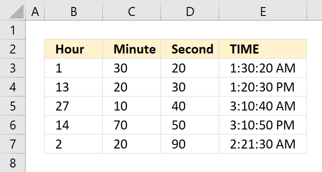
What is the TIME function?
The TIME function returns a decimal value between 0 (zero) representing 12:00:00 AM and 0.99988426 representing 11:59:59 P.M.
Formula in cell D3:
Table of Contents
1. TIME Function Syntax
TIME(hour, minute, second)
2. TIME Function Arguments
| hour | Required. A number between 0 and 32767 represents the hour. |
| minute | Required. A number between 0 and 32767 represents the minute. |
| second | Required. A number between 0 and 32767 represents the second. |
3. What is time in Excel?

Excel time value is a number equal to or larger than 0 (zero) and smaller than 1, formatted as a time value. One hour is 1/24, there are 24 hours in one day.
One minute is 1/1440, there are 1440 minutes in one day (60*24 = 1440). One second is 1/86400, there are 86400 seconds in one day (60*60*24 = 86400).
The following table shows whole hours, one hour is 1/24, 2 hours is 2/24, and so on.
0 - 12:00:00 AM
1/24 - 1:00:00 AM
2/24 - 2:00:00 AM
...
23/24 - 11:00:00 PM
24/24 - 12:00:00 AM
The time value is only the decimal part of a number, in other words, a value larger than or equal to 1 makes no difference, Excel uses only the decimal part of a number to create an Excel time value.
1.5 -> 0.5 -> 12:00:00 PM
The whole numbers represent dates in Excel. The whole number and the decimal part create a date and time value. Here is an example: 1.5 represents 1/1/1900 12:00 PM
4. TIME Function example
The TIME function creates an Excel time value meaning a number equal to or larger than 0 (zero) and smaller than 1 formatted as a time value.
Formula in cell E3:
Explaining formula
Step 1 - TIME function
TIME(hour, minute, second)
Step 2 - Populate arguments
TIME(hour, minute, second)
hour - B3
minute - C3
second - D3
Step 3 - Evaluate formula
TIME(1, 30, 20)
and returns 0.062731481 (1:30:20 AM).
1 hour = 1/24
30 min = 30/1440
20 sec = 20/86400
1/24 + 30/1440 + 20/86400 = 0.062731481
4.1 Time function - Hour value larger than 24

An hour value greater than 23 will be divided by 24 and the remaining hours will be returned by the function.
27/24 = 1.125 The decimal part is 0.125 and is equal to 3 hours. 3/24 = 0.125
4.2 Time function - Minute value larger than 59

A minute value equal to or greater than 60 will be divided by 60, the whole number is hours and the remaining minutes will be minutes.
119/60 is approx. 1.983333 The TIME function returns 1:59:00 AM. 0.983333 is approx. 59 minutes.
4.3 Time function - Seconds value larger than 59

A "second" value equal to or greater than 60 will be divided by 60 and added to minutes, the remaining seconds are returned.
7200/86400 is approx. 0.083333 which is the same as 120 minutes or 2 hours.
5. TIME Function - how to add hours

Formula in cell F3:
Alternative formula:
Note, the TIME function arguments are limited to 32767. Larger values return #NUM errors.
Explaining formula
Step 1 - Calculate hours in decimals
D3/24
becomes
5/24 equals 0.208333333.
Step 2 - Add time
B3+D3/24
becomes
0.979166667 + 5/24
becomes
0.979166667 + 0.208333333 equals 1.1875
6. TIME Function - how to add minutes

Formula in cell F3:
Alternative formula:
Note, the TIME function arguments are limited to 32767. Larger values return #NUM errors.
Explaining formula
Step 1 - Calculate hours in decimals
The division slash charcater lets you divide numbers in an Excel formula.
D3/24
becomes
5/1440 is approx. 0.0034722
Step 2 - Add time
The plus sign lets you add numbers in an Excel formula.
B3+D3/1440
becomes
0.979166667 + 5/1440
becomes
0.979166667 + 0.0034722
and is approx. 0.982638889
7. TIME Function - how to add seconds

Formula in cell F3:
Alternative formula:
Note, the TIME function arguments are limited to 32767. Larger values return #NUM errors.
Explaining formula
Step 1 - Calculate seconds in decimals
D3/24
becomes
5/86400
and is approx. 0.0000578
Step 2 - Add time
B3+D3/24
becomes
0.979166667 + 5/86400
becomes
0.979166667 + 0.0000578
and is approx. 0.979224537037037
8. How to calculate more than 24 hours?

The image above shows how to display an Excel time value larger than 1. This is possible using a different cell formatting code than the default one Excel uses.
- Select cell F3.
- Press CTRL + 1 to open the "Format Cells" dialog box.
- Select the "Custom" category.
- Use the following formatting code:
[h]:mm:ss - Press with left mouse button on OK button.
Explaining formula in cell F3
Step 1 - Calculate Excel time value
Cell F3 contains an Excel time value larger than 1.
B3+B5/24
becomes
0.979166666666667 + B5/24
becomes
0.979166666666667 + 60/24
becomes
0.979166666666667 + 2.5
and returns 3.47916666666667 in cell F3. Cell F3 is formatted using the following cell formatting code: [h]:mm:ss which shows 83:30:00 in cell F3.
Step 2 - Verify calculation
We can easily verify the calculation.
3*24 = 72 hours
0.47916666666667 * 24 equals 11.5 hours.
72 + 11.5 = 83.5 hours -> 83:30:00
9. Convert time to 24 hour clock

The TEXT functionlets you convert AM/PM to a 24 hour clock.
Formula in cell D3:
Explaining formula
Step 1 - TEXT function
The TEXT function converts a value to text in a specific number format.
TEXT(value, format_text)
| value | The string you want to format. You can use a cell reference here or use a text string. |
| format_text | Formatting code allows you to change the way, for example, a date or a number is displayed to the Excel user. |
Step 2 - Populate TEXT function arguments
TEXT(value, format_text)
value - B3
format_text - "hh:mm:ss"
hh - hours using two digits
mm - minutes (two digits)
ss - seconds (two digits)
Step 3 - Evaluate TEXT function
TEXT(B3,"hh:mm:ss")
becomes
TEXT(0.0627314814814815, "hh:mm:ss")
and returns 01:30:20.
1/24 + 30/1440 + 20/86400 equals 0.0627314814814815.
6. How to use the TIMEVALUE function
What is the TIMEVALUE function?
The TIMEVALUE function returns a decimal number representing an Excel time value, based on a text string. Excel uses decimal numbers between 0 and 0.99988426 formatted as time. 0 (zero) is 12:00:00 AM and 0.99988426 is 11:59:59 P.M.
The TIMEVALUE function in Excel is rarely needed to convert values in formulas. Excel automatically handles conversion of numbers, text, logical values, and error values as required. TIMEVALUE function is provided for compatibility with other spreadsheet applications. In most cases, Excel will format values correctly without requiring the TIMEVALUE function function.
Only use TIMEVALUE function if you find Excel is not properly converting a value to text in a specific formula. In general, you can avoid using it entirely since Excel auto-converts types seamlessly in most situations.
What is an Excel time value?
Excel time is actually a decimal number ranging between 0 and 1 in Excel and then formatted as time.
For example, 12:00 PM is represented as 0.5 because it is half of a day, you can verify this by typing 12:00 PM in a cell and then change the cell formatting to general. This will show the value as Excel interprets it.
Does the TIMEVALUE function ignore dates?
Yes, the TIMEVALUE function ignores the date part , example "22-Aug-2019 6:35 PM" returns 0.774305556 which is equal to "6:35 PM".
How does Excel recognize time values?
Excel recognizes certain text strings like "6:45 PM" as valid time values. A recognized time value is right aligned in the cell just like a regular number, shown in the image below in cell B2.
A time number that is not recognized is left aligned which is demonstrated in cell B4 in the image above. This visual feedback lets you easily spot values that need closer inspection.
How to show the decimal value as an Excel time value?

- Select the cell containing the decimal value.
- Press CTRL + 1 to open the "Format Cells" dialog box shown in the image above.
- Select category "Time".
- Select a type.
- Press with left mouse button on the "OK" button.

Why convert time values to decimal numbers?
The conversion allows you to perform arithmetic operations to time values, this works only if the time value is represented as a numerical value.
This lets you add or subtract, for instance, hours, minutes, and seconds easily using simple Excel formulas. It also lets you perform average, median, and other calculations using specific Excel functions.
TIMEVALUE function Syntax
TIMEVALUE(time_text)
TIMEVALUE function Arguments
| time_text | Required. A text string within quotation marks that represent time, for example "03:23 PM" or "22:21". |
TIMEVALUE function example
The image above demonstrates the TIMEVALUE function in cells B3 to B8, it converts time values as text values to decimal numbers.
Formula in cell B3:
The decimal numbers shown in cells B3 to B8 are the actual Excel time representation of:
- 1:48 AM
- 6:11 PM
- 9:58 AM
- 11:59:59 PM
- 0:00 AM
- 12:00 PM
7. How to use the TODAY function
What is the TODAY function?
The TODAY function returns the Excel date (serial number) of the current date.
What is a volatile function?
The TODAY function is a volatile function, it updates or recalculates every time the worksheet is recalculated. This may slow down your workbook calculations considerably if there are many formulas that depend on the TODAY function.
It may also slow down your worksheet/workbook if you have many volatile functions.
When is the worksheet calculated?
Cells containing non volatile functions are only calculated once or until you force a recalculation, however, volatile functions are recalculated each time you type in a cell and press enter.
Can you stop recalculating a worksheet?
Yes, you can change a setting to manual recalculations.
- Go to tab "Formulas".
- Press with left mouse button on the "Calculation Options" button, a popup menu appears.
- Press with mouse on "Manual".
This stops the automatic recalculations.
How to force a recalculation?
Pressing F9 key will recalculate or refresh all the formulas and values in every worksheet of every workbook you have open.
Pressing Shift+F9 will only recalculate the formulas and values on the single worksheet you're currently viewing or active.
Pressing Ctrl+Alt+F9 is the quickest way to force a full recalculation of absolutely everything in all open workbooks, even if nothing has changed. It ignores whether changes were made or not and completely recomputes.
Are there more volatile functions in Excel?
Yes. OFFSET, TODAY, RAND, NOW among others.
| Function | Syntax | Description |
|---|---|---|
| OFFSET | OFFSET(reference, rows, cols) | Returns a cell offset from a reference cell. |
| NOW | NOW() | Returns the current time. |
| RAND | RAND() | Returns a random decimal between 0 and 1. |
| RANDARRAY | RANDARRAY([rows], [columns], [min], [max], [whole_number]) | Returns an array with random numbers. |
| RANDBETWEEN | RANDBETWEEN(bottom, top) | Returns a random whole number between bottom and top |
Note, that conditional formatting is extremely volatile or super-volatile meaning it is recalculated as you scroll through a worksheet.
What are dates in Excel?
Dates are stored numerically but formatted to display in human-readable date/time formats, this enables Excel to do work with dates in calculations.
For example, dates are stored as sequential serial numbers with 1 being January 1, 1900 by default. The integer part (whole number) represents the date the decimal part represents the time.
This allows dates to easily be formatted to display in many date/time formats like mm/dd/yyyy, dd/mm/yyyy and so on and still be part of calculations as long as the date is stored numerically in a cell.
You can try this yourself, type 10000 in a cell, press CTRL + 1 and change the cell's formatting to date, press with left mouse button on OK. The cell now shows 5/18/1927.
TODAY Function Syntax
TODAY()
TODAY Function Arguments
The TODAY function has no arguments
TODAY Function example
Formula in cell B4:
What does the TODAY function return?
The Excel date the TODAY function returns is a serial number that Excel recognizes and can be filtered, sorted and used in other date calculations.
Excel dates are actually serial numbers formatted as dates, 1/1/1900 is 1 and 2/2/2018 is 43133. There are 43132 days between 2/2/2018 and 1/1/1900.
You can try this yourself, type 10000 in a cell, press CTRL + 1 and change the cell's formatting to date, press with left mouse button on OK. The cell now shows 5/18/1927.
Filter the upcoming dates for next week

This example demonstrates a formula that extracts records from cell range B3:C18 if the dates fall during the next seven days. The formula automatically changes the date
Excel 365 formula in cell E5:
This formula works only in Excel 365, the FILTER function may return multiple values that automatically spills to cells below.
Explaining formula
An Excel date is a serial number that Excel recognizes and can be filtered, sorted and used in other date calculations.
Excel dates are actually serial numbers formatted as dates, 1/1/1900 is 1 and 2/2/2018 is 43133. There are 43132 days between 2/2/2018 and 1/1/1900.
You can try this yourself, type 10000 in a cell, press CTRL + 1 and change the cell's formatting to date, press with left mouse button on OK. The cell now shows 5/18/1927.
Step 1 - Add 7 days to today's date
The plus sign + lets you perform addition in an Excel formula.
TODAY()+7
becomes
45241+7
equals 45248 (11/18)
Step 2 - Check dates smaller than today plus 7 days
The less than sign. larger than sign, and the equal sign are comparison operators that let you create logical expressions. The logical expression returns the boolean value, TRUE or FALSE.
B3:B18<=TODAY()+7
becomes
{45249; 45244; 45234; 45245; 45245; 45251; 45241; 45241; 45252; 45247; 45241; 45251; 45252; 45253; 45240; 45240}<=45248
and returns
{TRUE; TRUE; TRUE; TRUE; TRUE; FALSE; TRUE; TRUE; FALSE; TRUE; TRUE; FALSE; FALSE; FALSE; TRUE; TRUE}
Step 3 - Check dates later than or equal to today
B3:B18>=TODAY()
{45249; 45244; 45234; 45245; 45245; 45251; 45241; 45241; 45252; 45247; 45241; 45251; 45252; 45253; 45240; 45240}<=45241
and returns
{TRUE; TRUE; FALSE; TRUE; TRUE; TRUE; FALSE; FALSE; TRUE; TRUE; FALSE; TRUE; TRUE; TRUE; FALSE; FALSE}
Step 4 - Multiply boolean values to perform AND logic
The asterisk character lets you multiply numbers and boolean values in an Excel formula. The numerical equivalent to boolean value TRUE is 1 and FALSE is 0 (zero)
(B3:B18<=TODAY()+7)*(B3:B18>=TODAY())
becomes
{TRUE; TRUE; TRUE; TRUE; TRUE; FALSE; TRUE; TRUE; FALSE; TRUE; TRUE; FALSE; FALSE; FALSE; TRUE; TRUE} * {TRUE; TRUE; FALSE; TRUE; TRUE; TRUE; FALSE; FALSE; TRUE; TRUE; FALSE; TRUE; TRUE; TRUE; FALSE; FALSE}
and returns
{1;1;0;1;1;0;0;0;0;1;0;0;0;0;0;0}
Step 5 - Filter records
The FILTER function extracts values/rows based on a condition or criteria.
Function syntax: FILTER(array, include, [if_empty])
FILTER(B3:C18,(B3:B18<=TODAY()+7)*(B3:B18>=TODAY()))
becomes
FILTER(B3:C18,{1;1;0;1;1;0;0;0;0;1;0;0;0;0;0;0})
and returns the following array in cell E5 and spills to adjacent cells to the right and below as far as needed.
{45249, "#001"; 45244, "#007"; 45245, "#016"; 45245, "#012"; 45247, "#009"}
8. How to use the WEEKDAY function
What is the WEEKDAY function?
The WEEKDAY function converts a date to a number from 1 to 7 corresponding to a weekday or weekend day. You can customize the function so the week starts with any weekday.
Table of Contents
1. Introduction
What is a weekday?
A weekday refers to the days of the week that are typically considered work days or business days in parts of the world that follow a Monday to Friday work week. Saturday and Sunday are usually considered weekend days, not weekdays.
What is a weekend day?
A weekend day is Saturday and Sunday in most calendars. A weekend day refers to the days of the week that are typically considered non-work days in parts of the world that follow a standard Monday to Friday work week.
2. WEEKDAY Function Syntax
WEEKDAY(serial_number,[return_type])
3. WEEKDAY Function Arguments
| serial_number | Required. The Excel date value you want to extract the WEEKDAY number from. |
| return_type | Optional. Determines the type of return value, see table below. |
Why is the date a serial number?
The Excel date system uses a serial number system to represent dates, where each day is represented by a unique number. This system makes it easier to perform calculations and comparisons with dates. The serial number for January 1, 1900 is 1, and each subsequent day is represented by a serial number that increases by 1.
| Return_type | Number returned |
| 1 or omitted | Numbers 1 to 7 for Sunday to Saturday. |
| 2 | Numbers 1 to 7 for Monday to Sunday. |
| 3 | Numbers 0 to 6 for Monday to Sunday. |
| 11 | Numbers 1 to 7 for Monday to Sunday. |
| 12 | Numbers 1 to 7 for Tuesday to Monday. |
| 13 | Numbers 1 to 7 for Wednesday to Tuesday. |
| 14 | Numbers 1 to 7 for Thursday to Wednesday. |
| 15 | Numbers 1 to 7 for Friday to Thursday . |
| 16 | Numbers 1 to 7 for Saturday to Friday . |
| 17 | Numbers 1 to 7 for Sunday to Saturday. |
4. Video
5. WEEKDAY function example
The WEEKDAY function shown in cell D3 in the image above calculates a number based on a date. The number represents a given weekday based on the provided value in the second argument.
The formula below has no second argument, it defaults to 1 meaning the week begins with a Sunday.
Formula in cell D3:
6. WEEKDAY function not working
- Check your spelling.
- Check that you are using a valid Excel date.
- Check the number of arguments.
7. WEEKDAY function - show name

Formula in cell C3:
=TEXT(B3, "DDDD")
Step 1 - TEXT function
The TEXT function lets you format values.
TEXT(value, format_text)
value - The string you want to format. You can use a cell reference here or use a text string.
format_text - Formatting code allowing you to change the way, for example, a date or a number is displayed to the Excel user.
Step 2 - Populate arguments
The TEXT function has two arguments.
value - B3
format_text - "dddd"
"dddd" returns the weekday. Lower and upper case letters make no difference.
Check out this article to learn more about formatting codes in the TEXT function.
Step 3 - Evaluate TEXT function
TEXT(B3, "dddd")
becomes
TEXT(43263, "dddd")
and returns "Tuesday".

Formula in cell C4:
=INDEX({"Sunday";"Monday";"Tuesday";"Wednesday";"Thursday";"Friday";"Saturday"}, WEEKDAY(B4,1))
Explaining formula
Step 1 - Calculate number representing a weekday
WEEKDAY(B4,1)
becomes
WEEKDAY(43184, 1)
and returns 1.
Step 2 - Return weekday name based on position in array
The INDEX function returns a value in a cell range or array based on a row and column number (optional).
INDEX(array, [row_num], [column_num], [area_num])
INDEX({"Sunday";"Monday";"Tuesday";"Wednesday";"Thursday";"Friday";"Saturday"}, WEEKDAY(B4,1))
becomes
INDEX({"Sunday";"Monday";"Tuesday";"Wednesday";"Thursday";"Friday";"Saturday"}, 1)
and returns "Sunday". "Sunday" is the first value in the array.
8. Count days between two given weekdays and two dates

The image above shows an Excel 365 formula that counts days between two dates and also if they are between two given weekdays.
The start date is specified in cell K3, end date is in cell K4. The start weekday is 3 which represents Tuesday, the table in J11:K18 shows the numbers and corresponding weekday names. The end weekday is 5 which represents Thursday.
The calendar in cell range B4:H9 shows which days (bolded) meet the criteria. Cell K9 displays the result, there are six bolded days in the calendar.
Excel 365 dynamic array formula in cell K6:
=LET(x,SEQUENCE(K4-K3+1,,0),y,WEEKDAY(x+K3,1),COUNT(FILTER(x,(y<=K7)*(y>=K6))))
Explaining formula
COUNT(FILTER(SEQUENCE(K4-K3+1,,0),(WEEKDAY(SEQUENCE(K4-K3+1,,0)+K3,1)<=K7)*(WEEKDAY(SEQUENCE(K4-K3+1,,0)+K3,1)>=K6)))
Step 1 - Calculate the number of days and add one
The minus and plus signs let you perform arithmetic operations in an Excel formula
K4-K3+1
44648 - 44631 +1
equals 18.
Step 2 - Create a sequence of numbers from 0 to 18
The SEQUENCE function creates a list of sequential numbers to a cell range or array. It is located in the Math and trigonometry category and is only available to Excel 365 subscribers.
SEQUENCE(rows, [columns], [start], [step])
SEQUENCE(K4-K3+1,,0)
becomes
SEQUENCE(18,,0)
and returns
{0; 1; 2; 3; 4; 5; 6; 7; 8; 9; 10; 11; 12; 13; 14; 15; 16; 17}.
Step 3 - Add date to sequence of numbers
The plus sign lets you perform add numbers in an Excel formula.
SEQUENCE(K4-K3+1,,0)+K3
becomes
{0; 1; 2; 3; 4; 5; 6; 7; 8; 9; 10; 11; 12; 13; 14; 15; 16; 17} + 44631
and returns
{44631; 44632; 44633; 44634; 44635; 44636; 44637; 44638; 44639; 44640; 44641; 44642; 44643; 44644; 44645; 44646; 44647; 44648}.
Step 4 - Calculate weekday
WEEKDAY(SEQUENCE(K4-K3+1,,0)+K3,1)
becomes
WEEKDAY({44631; 44632; 44633; 44634; 44635; 44636; 44637; 44638; 44639; 44640; 44641; 44642; 44643; 44644; 44645; 44646; 44647; 44648},1)
and returns
{6; 7; 1; 2; 3; 4; 5; 6; 7; 1; 2; 3; 4; 5; 6; 7; 1; 2}.
Step 5 - Check if number is less than seven
The less than and larger than characters let you check if a value is smaller or larger than a condition, the result is a boolean value TRUE or FALSE. The equal sign and the less than character combined compare if values are equal or smaller than a condition.
WEEKDAY(SEQUENCE(K4-K3+1,,0)+K3,1)<=K7
becomes
{6; 7; 1; 2; 3; 4; 5; 6; 7; 1; 2; 3; 4; 5; 6; 7; 1; 2}<=5
and returns
{FALSE; FALSE; TRUE; TRUE; TRUE; TRUE; TRUE; FALSE; FALSE; TRUE; TRUE; TRUE; TRUE; TRUE; FALSE; FALSE; TRUE; TRUE}.
Step 6 - Check if weekday is larger than one
WEEKDAY(SEQUENCE(K4-K3+1,,0)+K3,1)>=K6
becomes
{6; 7; 1; 2; 3; 4; 5; 6; 7; 1; 2; 3; 4; 5; 6; 7; 1; 2}>=3
and returns
{TRUE; TRUE; FALSE; FALSE; TRUE; TRUE; TRUE; TRUE; TRUE; FALSE; FALSE; TRUE; TRUE; TRUE; TRUE; TRUE; FALSE; FALSE}.
Step 7 - Multiply arrays
The asterisk character lets you multiple values in an Excel formula. Multiplying boolean values always return their numerical equivalents.
TRUE -> 1
FALSE -> 0 (zero)
(WEEKDAY(SEQUENCE(K4-K3+1,,0)+K3,1)<7)*(WEEKDAY(SEQUENCE(K4-K3+1,,0)+K3,1)>1)
becomes
{FALSE; FALSE; TRUE; TRUE; TRUE; TRUE; TRUE; FALSE; FALSE; TRUE; TRUE; TRUE; TRUE; TRUE; FALSE; FALSE; TRUE; TRUE}*{TRUE; TRUE; FALSE; FALSE; TRUE; TRUE; TRUE; TRUE; TRUE; FALSE; FALSE; TRUE; TRUE; TRUE; TRUE; TRUE; FALSE; FALSE}
and returns
{0; 0; 0; 0; 1; 1; 1; 0; 0; 0; 0; 1; 1; 1; 0; 0; 0; 0}.
Step 8 - Filter numbers based on condition
The FILTER function is a new function available to Excel 365 subscribers. It lets you extract values based on a condition or criteria.
FILTER(array, include, [if_empty])
FILTER(SEQUENCE(K4-K3+1,,0),(WEEKDAY(SEQUENCE(K4-K3+1,,0)+K3,1)<7)*(WEEKDAY(SEQUENCE(K4-K3+1,,0)+K3,1)>1))
becomes
FILTER({0; 1; 2; 3; 4; 5; 6; 7; 8; 9; 10; 11; 12; 13; 14; 15; 16; 17},{0; 0; 0; 0; 1; 1; 1; 0; 0; 0; 0; 1; 1; 1; 0; 0; 0; 0})
and returns
{4; 5; 6; 11; 12; 13}.
Step 9 - Count numbers in the array
The COUNT function counts all numbers in a cell range or array.
COUNT(value1, [value2], ...)
COUNT(FILTER(SEQUENCE(K4-K3+1,,0),(WEEKDAY(SEQUENCE(K4-K3+1,,0)+K3,1)<7)*(WEEKDAY(SEQUENCE(K4-K3+1,,0)+K3,1)>1)))
becomes
COUNT({4; 5; 6; 11; 12; 13})
and returns 6. There are six numbers in the array.
Step 10 - Shorten formula
The LET function allows you to name intermediate calculation results which can shorten formulas considerably and improve performance.
LET(name1, name_value1, calculation_or_name2, [name_value2, calculation_or_name3...])
LET(x, SEQUENCE(K4-K3+1, , 0), y, WEEKDAY(x+K3, 1), COUNT(FILTER(x, (y<7)*(y>1))))
x - SEQUENCE(K4-K3+1,,0)
y - WEEKDAY(x+K3,1)
9. How to calculate a date based on specific weekday in a month
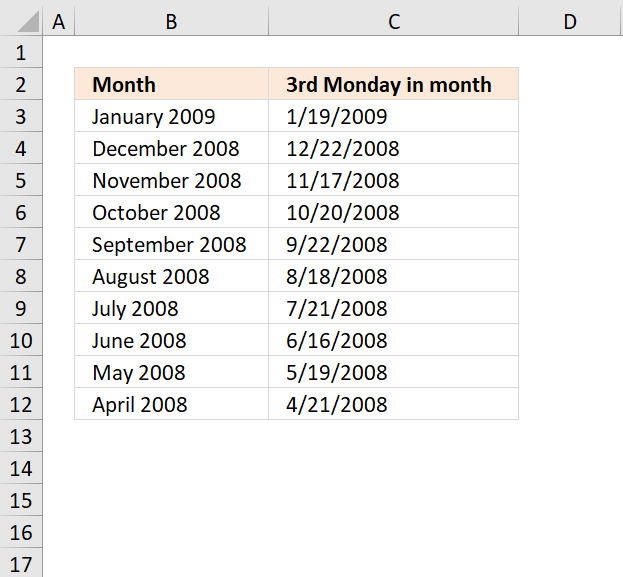
Question:
How to calculate the date of the third Monday of a given month?
Answer:
Column B contains dates of the first date of a month, however, they are formatted as Month and year. This makes it possible to use the corresponding cell value in our formula.
Excel 365 dynamic array formula in cell C3:
Array formula in cell C3
To enter an array formula, type the formula in cell C3 then press and hold CTRL + SHIFT simultaneously, now press Enter once. Release all keys.
 The formula bar now shows the formula with a beginning and ending curly bracket telling you that you entered the formula successfully.
Don't enter the curly brackets yourself, they appear automatically.
Explaining array formula in cell C3
Step 1 - Create an array of numbers corresponding to days in month
The EOMONTH function calculates the last date in a given month, the DAY function then returns the day of that date.
ROW(INDIRECT( "$1:$"&DAY( EOMONTH(B3, 0))))-1)
becomes
ROW(INDIRECT( "$1:$"&DAY( EOMONTH(39814, 0))))-1)
becomes
ROW(INDIRECT( "$1:$"&DAY( 39844)))-1)
becomes
ROW(INDIRECT( "$1:$"&DAY( 39844)))-1)
becomes
ROW(INDIRECT("$1:$"&31))-1
The INDIRECT function converts a text string to a cell reference that an Excel function then can use.
ROW(INDIRECT($1:$31))-1
becomes
ROW($1:$31)-1
The ROW function then returns the row numbers of each cell in the cell reference.
ROW($1:$31)-1
becomes
{1; 2; 3; 4; 5; 6; 7; 8; 9; 10; 11; 12; 13; 14; 15; 16; 17; 18; 19; 20; 21; 22; 23; 24; 25; 26; 27; 28; 29; 30; 31} - 1
and returns {0; 1; 2; 3; 4; 5; 6; 7; 8; 9; 10; 11; 12; 13; 14; 15; 16; 17; 18; 19; 20; 21; 22; 23; 24; 25; 26; 27; 28; 29; 30}
Step 2 - Check if date is a Monday
The array in the step before is now going to be added to the first date in the given month.
WEEKDAY(B3 +ROW(INDIRECT( "$1:$"&DAY( EOMONTH(B3, 0))))-1)=2
becomes
WEEKDAY(B3 +{0; 1; 2; 3; 4; 5; 6; 7; 8; 9; 10; 11; 12; 13; 14; 15; 16; 17; 18; 19; 20; 21; 22; 23; 24; 25; 26; 27; 28; 29; 30})=2
becomes
WEEKDAY({39814; 39815; 39816; 39817; 39818; 39819; 39820; 39821; 39822; 39823; 39824; 39825; 39826; 39827; 39828; 39829; 39830; 39831; 39832; 39833; 39834; 39835; 39836; 39837; 39838; 39839; 39840; 39841; 39842; 39843; 39844})=2
It is worth mentioning that Excel treats dates as numbers. For example, number 1 is 1/1/1900 and 1/1/2000 is 36526. 1/2/2000 is 36527. The numbers you see above in the array are dates.
The WEEKDAY function converts the dates to their corresponding weekdays in numbers. 1 is Sunday and 7 is Saturday.
WEEKDAY({39814; 39815; 39816; 39817; 39818; 39819; 39820; 39821; 39822; 39823; 39824; 39825; 39826; 39827; 39828; 39829; 39830; 39831; 39832; 39833; 39834; 39835; 39836; 39837; 39838; 39839; 39840; 39841; 39842; 39843; 39844})=2
becomes
{5;6;7;1;2;3;4;5;6;7;1;2;3;4;5;6;7;1;2;3;4;5;6;7;1;2;3;4;5;6;7}=2
To identify Mondays in this array I will compare the numbers with 2.
{5;6;7;1;2;3;4;5;6;7;1;2;3;4;5;6;7;1;2;3;4;5;6;7;1;2;3;4;5;6;7}=2
returns the following boolean array:
{FALSE; FALSE; FALSE; FALSE; TRUE; FALSE; FALSE; FALSE; FALSE; FALSE; FALSE; TRUE; FALSE; FALSE; FALSE; FALSE; FALSE; FALSE; TRUE; FALSE; FALSE; FALSE; FALSE; FALSE; FALSE; TRUE; FALSE; FALSE; FALSE; FALSE; FALSE}
Boolean values are TRUE and FALSE.
Step 3 - Return corresponding date if Monday
The IF function lets you evaluate a logical expression and if TRUE one thing happens and if FALSE another thing happens.
The logical expression in this example evaluates to TRUE if date is a Monday.
IF(WEEKDAY(B3+ROW(INDIRECT("$1:$"&DAY(EOMONTH(B3,0))))-1)=2,B3+ROW(INDIRECT("$1:$"&DAY(EOMONTH(B3,0))))-1,"")
becomes
IF({FALSE; FALSE; FALSE; FALSE; TRUE; FALSE; FALSE; FALSE; FALSE; FALSE; FALSE; TRUE; FALSE; FALSE; FALSE; FALSE; FALSE; FALSE; TRUE; FALSE; FALSE; FALSE; FALSE; FALSE; FALSE; TRUE; FALSE; FALSE; FALSE; FALSE; FALSE},B3+ROW(INDIRECT("$1:$"&DAY(EOMONTH(B3,0))))-1,"")
If the value is TRUE then return the corresponding date. Since months have different number of days we must build an array that takes that into account.
It works just like the array we created in step 1.
IF({FALSE; FALSE; FALSE; FALSE; TRUE; FALSE; FALSE; FALSE; FALSE; FALSE; FALSE; TRUE; FALSE; FALSE; FALSE; FALSE; FALSE; FALSE; TRUE; FALSE; FALSE; FALSE; FALSE; FALSE; FALSE; TRUE; FALSE; FALSE; FALSE; FALSE; FALSE},B3+ROW(INDIRECT("$1:$"&DAY(EOMONTH(B3,0))))-1,"")
becomes
IF({FALSE; FALSE; FALSE; FALSE; TRUE; FALSE; FALSE; FALSE; FALSE; FALSE; FALSE; TRUE; FALSE; FALSE; FALSE; FALSE; FALSE; FALSE; TRUE; FALSE; FALSE; FALSE; FALSE; FALSE; FALSE; TRUE; FALSE; FALSE; FALSE; FALSE; FALSE},{39814; 39815; 39816; 39817; 39818; 39819; 39820; 39821; 39822; 39823; 39824; 39825; 39826; 39827; 39828; 39829; 39830; 39831; 39832; 39833; 39834; 39835; 39836; 39837; 39838; 39839; 39840; 39841; 39842; 39843; 39844},"")
and returns
{""; ""; ""; ""; 39818; ""; ""; ""; ""; ""; ""; 39825; ""; ""; ""; ""; ""; ""; 39832; ""; ""; ""; ""; ""; ""; 39839; ""; ""; ""; ""; ""}
Step 3 - Filter third Monday
The SMALL function lets you return the third largest number in array because we are looking for the third Monday in a given month.
SMALL(IF(WEEKDAY(B3 +ROW(INDIRECT( "$1:$"&DAY( EOMONTH(B3, 0))))-1)=2, B3+ROW( INDIRECT("$1:$"&DAY( EOMONTH(B3, 0))))-1, ""), 3)
becomes
SMALL({""; ""; ""; ""; 39818; ""; ""; ""; ""; ""; ""; 39825; ""; ""; ""; ""; ""; ""; 39832; ""; ""; ""; ""; ""; ""; 39839; ""; ""; ""; ""; ""}, 3)
and returns 39832 in cell C3 which is the same as 1/19/2009 if formatted as a date in Excel.
Get Excel *.xlsx file
9. How to use the WEEKNUM function
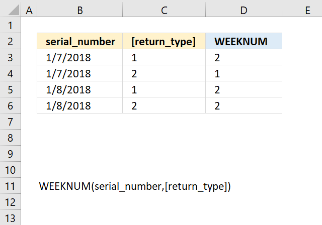
What is the WEEKNUM function?
The WEEKNUM function calculates a given date's week number based on a return_type parameter that determines which day the week begins.
Table of Contents
1. Introduction
What is a week?
A week is a time unit used to represent the cycle of seven days in the Gregorian calendar. A week consists of seven consecutive days, typically beginning on Sunday, Monday or Saturday depending on country and calendar system.
Each week cycles through the seven days of the week - Sunday, Monday, Tuesday, Wednesday, Thursday, Friday, and Saturday.
How many weeks in a year?
Week numbers range from 1 to 52 for most years. Some years have 53 weeks if the 1st week starts very early in the previous year.
Is a week the same in all parts of the world?
No, the definition and numbering of a week is not the same in all parts of the world.
There are some key differences:
- Start of week - Some calendars start the week on Sunday, others on Monday.
- Week numbering - The rules for when Week 1 begins in a year vary between calendars.
- ISO 8601 standard - This internationally recognizes Monday as start of week and has a consistent week numbering definition.
- Cultural variations - Some cultures or religions use different definitions of a week. For example, the Jewish calendar week starts on Sunday.
What is a week number?
A week number refers to the ordinal numbering of weeks in a calendar year.
ISO 8601 is the international standard for week numbering. Week numbers provide an alternative to the month/day system for identifying dates. They are commonly used in work/school calendars, schedules, timetables, payment periods, etc.
When does week numbers start?
Week 1 is the first week of the year that contains at least 4 days of the new year.
What is the difference between the WEKNUM function and the ISOWEEKNUM function?
ISOWEEKNUM follows the ISO 8601 international standard for week numbering, while WEEKNUM is based on a more localized definition.
ISOWEEKNUM always starts weeks on Monday and Week 1 is the first week with 4+ days in the new year. WEEKNUM can start weeks on Sunday or Monday based on system settings.
| Region | First Day of Week | Week Numbering |
|---|---|---|
| Europe | Monday | ISO 8601 (Week 1 is first with 4+ days in new year) |
| North America | Sunday | Other |
| South America | Monday | ISO 8601 |
| Asia | Monday or Sunday | Varies by country, ISO and others |
| Middle East | Saturday | Varies by country |
| Africa | Sunday or Monday | ISO 8601 or others |
Most regions follow ISO 8601 now but there are still some variations.
2. WEEKNUM function Syntax
WEEKNUM(serial_number,[return_type])
3. WEEKNUM function Arguments
| serial_number | Required. A date. If you enter the date in the function then use the DATE function to calculate the correct serial_number. |
| [return_type] | Optional. A number determining which day the week begins. If omitted, 1 is used. |
The following table shows how the WEEKNUM function defines a week if [return_type] argument is specified.
| [return_type] | Week starts on | System |
| 1 | Sunday | 1 |
| 2 | Monday | 1 |
| 11 | Monday | 1 |
| 12 | Tuesday | 1 |
| 13 | Wednesday | 1 |
| 14 | Thursday | 1 |
| 15 | Friday | 1 |
| 16 | Saturday | 1 |
| 17 | Sunday | 1 |
| 21 | Monday | 2 |
You also have the option to choose which system to use, see the [return_type] argument.
| System 1 | Week 1 is the week that contains January 1. |
| System 2 | Week 1 is the week that contains the first Thursday of the year. (European week numbering system). |
4. WEEKNUM function example
Formula in cell D3:
5. Extract week ranges based on a given date range

The formula in cell B7 and C7 extracts whole weeks within the given date range in cell B3 and C3.
The following array formula in cell C7 extracts weeks that begin on a Sunday:
Formula in cell B7:
To enter an array formula, type the formula in a cell then press and hold CTRL + SHIFT simultaneously, now press Enter once. Release all keys.
The formula bar now shows the formula with a beginning and ending curly bracket telling you that you entered the formula successfully. Don't enter the curly brackets yourself.
Excel 365 dynamic array formula in cell B7:
Explaining formula in cell C7
Step 1 - Create array 1 to n
The INDEX function creates a cell reference with the same number of rows as there are dates in the date range.
The ROW function then converts the cell range to an array of corresponding row numbers.
ROW($A$1:INDEX($A$1:$A$1000, $C$3-$B$3))
becomes
ROW($A$1:INDEX($A$1:$A$1000, 40633-40569))
becomes
ROW($A$1:INDEX($A$1:$A$1000, 64))
becomes
ROW($A$1:$A$64)
and returns
{1; 2; 3; 4; 5; 6; 7; 8; 9; 10; 11; 12; 13; 14; 15; 16; 17; 18; 19; 20; 21; 22; 23; 24; 25; 26; 27; 28; 29; 30; 31; 32; 33; 34; 35; 36; 37; 38; 39; 40; 41; 42; 43; 44; 45; 46; 47; 48; 49; 50; 51; 52; 53; 54; 55; 56; 57; 58; 59; 60; 61; 62; 63; 64}
Step 2 - Create dates within date range
The next step subtracts the array with 1 and adds the Excel date number.
$B$3+(ROW($A$1:INDEX($A$1:$A$1000, $C$3-$B$3))-1)
becomes
$B$3+({1; 2; 3; 4; 5; 6; 7; 8; 9; 10; 11; 12; 13; 14; 15; 16; 17; 18; 19; 20; 21; 22; 23; 24; 25; 26; 27; 28; 29; 30; 31; 32; 33; 34; 35; 36; 37; 38; 39; 40; 41; 42; 43; 44; 45; 46; 47; 48; 49; 50; 51; 52; 53; 54; 55; 56; 57; 58; 59; 60; 61; 62; 63; 64}-1)
becomes
$B$3+{0; 1; 2; 3; 4; 5; 6; 7; 8; 9; 10; 11; 12; 13; 14; 15; 16; 17; 18; 19; 20; 21; 22; 23; 24; 25; 26; 27; 28; 29; 30; 31; 32; 33; 34; 35; 36; 37; 38; 39; 40; 41; 42; 43; 44; 45; 46; 47; 48; 49; 50; 51; 52; 53; 54; 55; 56; 57; 58; 59; 60; 61; 62; 63}
becomes
40569+{0; 1; 2; 3; 4; 5; 6; 7; 8; 9; 10; 11; 12; 13; 14; 15; 16; 17; 18; 19; 20; 21; 22; 23; 24; 25; 26; 27; 28; 29; 30; 31; 32; 33; 34; 35; 36; 37; 38; 39; 40; 41; 42; 43; 44; 45; 46; 47; 48; 49; 50; 51; 52; 53; 54; 55; 56; 57; 58; 59; 60; 61; 62; 63}
and returns
{40569; 40570; 40571; 40572; 40573; 40574; 40575; 40576; 40577; 40578; 40579; 40580; 40581; 40582; 40583; 40584; 40585; 40586; 40587; 40588; 40589; 40590; 40591; 40592; 40593; 40594; 40595; 40596; 40597; 40598; 40599; 40600; 40601; 40602; 40603; 40604; 40605; 40606; 40607; 40608; 40609; 40610; 40611; 40612; 40613; 40614; 40615; 40616; 40617; 40618; 40619; 40620; 40621; 40622; 40623; 40624; 40625; 40626; 40627; 40628; 40629; 40630; 40631; 40632}
Step 3 - Convert dates to weekdays
The TEXT function converts the dates to weekdays.
TEXT($B$3+(ROW($A$1:INDEX($A$1:$A$1000, $C$3-$B$3))-1), "DDD")
becomes
TEXT({40569; 40570; 40571; 40572; 40573; 40574; 40575; 40576; 40577; 40578; 40579; 40580; 40581; 40582; 40583; 40584; 40585; 40586; 40587; 40588; 40589; 40590; 40591; 40592; 40593; 40594; 40595; 40596; 40597; 40598; 40599; 40600; 40601; 40602; 40603; 40604; 40605; 40606; 40607; 40608; 40609; 40610; 40611; 40612; 40613; 40614; 40615; 40616; 40617; 40618; 40619; 40620; 40621; 40622; 40623; 40624; 40625; 40626; 40627; 40628; 40629; 40630; 40631; 40632}, "DDD")
and returns
{"Wed"; "Thu"; "Fri"; "Sat"; "Sun"; "Mon"; "Tue"; "Wed"; "Thu"; "Fri"; "Sat"; "Sun"; "Mon"; "Tue"; "Wed"; "Thu"; "Fri"; "Sat"; "Sun"; "Mon"; "Tue"; "Wed"; "Thu"; "Fri"; "Sat"; "Sun"; "Mon"; "Tue"; "Wed"; "Thu"; "Fri"; "Sat"; "Sun"; "Mon"; "Tue"; "Wed"; "Thu"; "Fri"; "Sat"; "Sun"; "Mon"; "Tue"; "Wed"; "Thu"; "Fri"; "Sat"; "Sun"; "Mon"; "Tue"; "Wed"; "Thu"; "Fri"; "Sat"; "Sun"; "Mon"; "Tue"; "Wed"; "Thu"; "Fri"; "Sat"; "Sun"; "Mon"; "Tue"; "Wed"}
Step 4 - Extract all Sundays
The IF function has three arguments, the first one must be a logical expression. If the expression evaluates to TRUE then one thing happens (argument 2) and if FALSE another thing happens (argument 3).
IF(TEXT($B$3+(ROW($A$1:INDEX($A$1:$A$1000, $C$3-$B$3))-1), "DDD")="Sat", $B$3+(ROW($A$1:INDEX($A$1:$A$1000, $C$3-$B$3))-1), "")
becomes
IF({"Wed"; "Thu"; "Fri"; "Sat"; "Sun"; "Mon"; "Tue"; "Wed"; "Thu"; "Fri"; "Sat"; "Sun"; "Mon"; "Tue"; "Wed"; "Thu"; "Fri"; "Sat"; "Sun"; "Mon"; "Tue"; "Wed"; "Thu"; "Fri"; "Sat"; "Sun"; "Mon"; "Tue"; "Wed"; "Thu"; "Fri"; "Sat"; "Sun"; "Mon"; "Tue"; "Wed"; "Thu"; "Fri"; "Sat"; "Sun"; "Mon"; "Tue"; "Wed"; "Thu"; "Fri"; "Sat"; "Sun"; "Mon"; "Tue"; "Wed"; "Thu"; "Fri"; "Sat"; "Sun"; "Mon"; "Tue"; "Wed"; "Thu"; "Fri"; "Sat"; "Sun"; "Mon"; "Tue"; "Wed"}="Sun", $B$3+(ROW($A$1:INDEX($A$1:$A$1000, $C$3-$B$3))-1), "")
becomes
IF({FALSE; FALSE; FALSE; FALSE; TRUE; FALSE; FALSE; FALSE; FALSE; FALSE; FALSE; TRUE; FALSE; FALSE; FALSE; FALSE; FALSE; FALSE; TRUE; FALSE; FALSE; FALSE; FALSE; FALSE; FALSE; TRUE; FALSE; FALSE; FALSE; FALSE; FALSE; FALSE; TRUE; FALSE; FALSE; FALSE; FALSE; FALSE; FALSE; TRUE; FALSE; FALSE; FALSE; FALSE; FALSE; FALSE; TRUE; FALSE; FALSE; FALSE; FALSE; FALSE; FALSE; TRUE; FALSE; FALSE; FALSE; FALSE; FALSE; FALSE; TRUE; FALSE; FALSE; FALSE}, {40569; 40570; 40571; 40572; 40573; 40574; 40575; 40576; 40577; 40578; 40579; 40580; 40581; 40582; 40583; 40584; 40585; 40586; 40587; 40588; 40589; 40590; 40591; 40592; 40593; 40594; 40595; 40596; 40597; 40598; 40599; 40600; 40601; 40602; 40603; 40604; 40605; 40606; 40607; 40608; 40609; 40610; 40611; 40612; 40613; 40614; 40615; 40616; 40617; 40618; 40619; 40620; 40621; 40622; 40623; 40624; 40625; 40626; 40627; 40628; 40629; 40630; 40631; 40632}, "")
and returns
{""; ""; ""; ""; 40573; ""; ""; ""; ""; ""; ""; 40580; ""; ""; ""; ""; ""; ""; 40587; ""; ""; ""; ""; ""; ""; 40594; ""; ""; ""; ""; ""; ""; 40601; ""; ""; ""; ""; ""; ""; 40608; ""; ""; ""; ""; ""; ""; 40615; ""; ""; ""; ""; ""; ""; 40622; ""; ""; ""; ""; ""; ""; 40629; ""; ""; ""}
Step 5 - Find n-th Sunday within range
To be able to return a new value in a cell each I use the SMALL function to filter date numbers from smallest to largest.
SMALL(IF(TEXT($B$3+(ROW($A$1:INDEX($A$1:$A$1000, $C$3-$B$3))-1), "DDD")="Sat", $B$3+(ROW($A$1:INDEX($A$1:$A$1000, $C$3-$B$3))-1), ""),ROWS($A$1:A2))
becomes
SMALL({""; ""; ""; ""; 40573; ""; ""; ""; ""; ""; ""; 40580; ""; ""; ""; ""; ""; ""; 40587; ""; ""; ""; ""; ""; ""; 40594; ""; ""; ""; ""; ""; ""; 40601; ""; ""; ""; ""; ""; ""; 40608; ""; ""; ""; ""; ""; ""; 40615; ""; ""; ""; ""; ""; ""; 40622; ""; ""; ""; ""; ""; ""; 40629; ""; ""; ""}),ROWS($A$1:A2))
becomes
SMALL({""; ""; ""; ""; 40573; ""; ""; ""; ""; ""; ""; 40580; ""; ""; ""; ""; ""; ""; 40587; ""; ""; ""; ""; ""; ""; 40594; ""; ""; ""; ""; ""; ""; 40601; ""; ""; ""; ""; ""; ""; 40608; ""; ""; ""; ""; ""; ""; 40615; ""; ""; ""; ""; ""; ""; 40622; ""; ""; ""; ""; ""; ""; 40629; ""; ""; ""}),2)
and returns 40580 formatted as 2/5/2011.
Step 6 - Return blank if error
The IFERROR function handles errors, it returns a specified value if formula returns an error. In this case it returns a blank "".
6. WEEKNUM function not working
The WEEKNUM function returns #NUM! error if:
- serial_number is out of range.
- [return_type] is out of range.
10. How to use the WORKDAY function
What is the WORKDAY function?
The WORKDAY function returns a date based on a start date and a given number of working days (nonweekend and nonholidays).
What is a workday?
A weekday that is not a weekend day or holiday. Typically Monday through Friday excluding any holiday dates.
Use the WEEKDAY function to determine if a date is a workday or a weekend day.
What is a holiday?
A day on which regular activities and work is suspended due to a cultural, religious or legal custom. Varies by country and region.
WORKDAY function Syntax
WORKDAY(start_date, days, [holidays])
WORKDAY function Arguments
| start_date | Required. |
| days | Required. Positive integer returns a date after the start_date (future) and negative integer returns a date before the start_date. |
| [holidays] | Optional. A list of holiday dates. |
WORKDAY function not working
The WORKDAY function returns
- #VALUE! error value if start_date or [holidays] are not a valid date.
- #NUM error if start_date plus days argument returns an invalid date.
(Excel can't handle dates before 1/1/1900.)
Use the DATE function to create valid Excel dates.
Example:
What is an Excel date?
An Excel date is a serial number that Excel recognizes and can be filtered, sorted and used in other date calculations.
Excel dates are actually serial numbers formatted as dates, 1/1/1900 is 1 and 2/2/2018 is 43133. There are 43132 days between 2/2/2018 and 1/1/1900.
You can try this yourself, type 10000 in a cell, press CTRL + 1 and change the cell's formatting to date, press with left mouse button on OK. The cell now shows 5/18/1927.
WORKDAY function example
This example demonstrates how to use the WORKDAY function to calculate a future date with the condition of being a workday excluding weekend days and holidays.
The start date is shown in cell C3 in the image above. The number of working days days is 12 and the function returns 1/17/2018. The formula in cell B8 is shown below, note that no holidays has been specified.
Formula in cell B8:
The image below shows the start date and the weekdays. The count is entered below dates that are workdays.
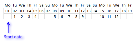
Note that there are no numbers below weekend days because they are not workdays. Counting 12 days after the start date and we get 1/17/2018.
WORKDAY function example - Negative days argument and a holiday
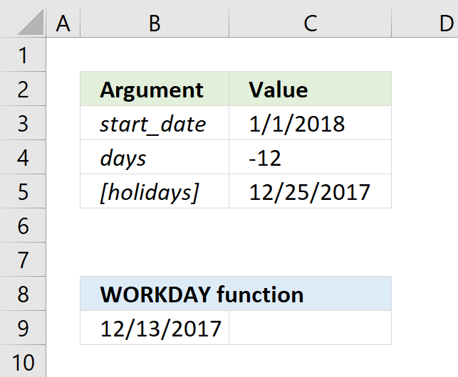
This example demonstrates the WORKDAY function with a negative day argument which means it calculates a workday before the start date instead of after the start date.
The start date is shown in cell C3 in the image above. The number of working days days is -12 and the function returns 12/13/2017. The formula in cell B8 is shown below, note that holiday 12/25/2017 has been specified.
Formula in cell B9:
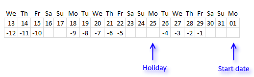
This example also shows no numbers below weekend days because they are not workdays, this applies to 12/25/2017 as well because it si specified as a holiday. Counting 12 days befoe the start date and we get 12/13/2017.
11. How to use the YEAR function
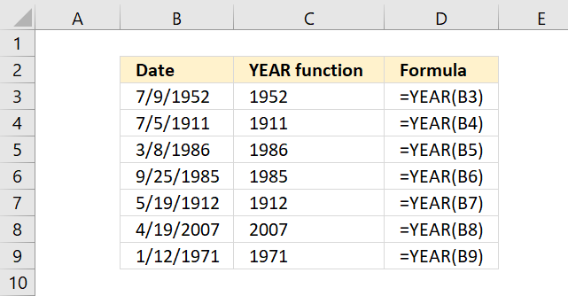
What is the YEAR function?
The YEAR function converts a date to a number representing the year in the date. The number is between 1900 and 9999.
Table of Contents
- YEAR function syntax
- YEAR function arguments
- YEAR function example
- Calculate year from date?
- How to extract the year from a text string
- YEAR function not working?
- Is date an Excel date?
- How to calculate years between dates?
- How to convert year to a date?
- Year and month
- Year and quarter
- Year as text
- Year and month to date?
- Year by week?
- The year begins on what weekday?
- Get Excel file
1. YEAR function syntax
YEAR(serial_number)
2. YEAR function arguments
serial_number - The date you want to extract the year out of.
Excel uses whole numbers as dates. January, 1 , 1900 is 1 and January, 1, 2000 is 36526. There are 36525 days between those two dates.
3. YEAR function example
Formula in cell C3:
4. How to calculate the year from a date?

The image above shows the YEAR function in cell C3, it calculates a 4-digit year number based on an Excel date (serial number).
Formula in cell C3:
5. How to extract the year from a text string
5.1 Date at the end of the text string

The image above demonstrates three different formulas that extract the year from a text string. Cell B3 is a text string with the four last characters being the year number.
Cell B4 has the year number between other characters both from the right and left. Cell C5 begins with the year numbers.
Formula in cell C3:
The RIGHT function extracts a given number of characters from a text string starting from right.
RIGHT(text, [num_chars])
text - B3
[num_chars] - 4

5.2 Date somewhere in the middle of the text string
Formula in cell C4:
The MID function returns a substring from a string based on the starting position and the number of characters you want to extract.
MID(text, start_num, num_chars)
text - B4
start_num - 5
num_chars - 4

The formula in cell C5 returns 1911.
5.3 Date at the beginning of the text string
Formula in cell C5:
The LEFT function extracts a given number of characters from a text string starting from the left.
LEFT(text, [num_chars])
text - B5
[num_chars] - 4

The formula in cell C5 returns 1986.
6. YEAR function not working?
6.1 YEAR function returns #NAME! error

The YEAR function is misspelled in cell C3, Excel returns a #NAME! error.
6.2 YEAR function returns #VALUE! error

Cell B3 contains a text string that the YEAR function in cell C3 doesn't recognize as a date.
Formula in cell C3:

This formula extracts the year from the string.
Formula in cell C3:
6.3 YEAR function returns #NUM! error

Cell B3 contains a string of letters that the YEAR function doesn't recognize as an Excel date. It returns #NUM! error.
Formula in cell C3:
The following formula extracts the year from the string.

Formula in cell C3:
7. Is date an Excel date?

The image above demonstrates three different values, Excel dates are right-aligned by default, text and general values are left-aligned by default.
However, numbers are also right-aligned by default. This can be confusing.
To really make sure Excel recognizes an Excel date go to tab "Home" on the ribbon. Select the cell you want to examine, now check the "Number Format".

Make sure Excel sees the dates as valid dates, see the image below.

Why do you want dates to be Excel dates?
You can't sort dates as text and general values properly, also calculations can't be made to text dates.
8. How to calculate years between dates?

The image above demonstrates a formula that returns the number of years between two given dates.
Formula in cell C3:
You can't use the YEAR function to calculate this, YEAR(C3) - YEAR(B3) returns 3 (2019-2016 equals 3), however, the correct result is 2.
Read more about the DATEDIF function.
9. How to convert year number to a date?

The picture above demonstrates a formula that returns an Excel date based on a year number specified in cell B3.
Formula in cell D3:
The formula in cell B6 is identical as the formula in cell D3, however, the cell is formatted to only show the year number. Read the next section to find out how to format.
9.1 How to format Excel date to yyyy

- Select cell B6.
- Press CTRL + 1 to open the "Format Cells" dialog box, see the image above.
- Select "Custom"
- Type: yyyy
- Press with left mouse button "OK" button.
Cell B6 is an Excel date showing only the year as a number.
10. Format Excel date to year and month

The image above shows a worksheet with the same date 6/28/2025 in cells B3:B8, however, cells B4:B8 are formatted differently.
- Select cell containing an Excel date.
- Press CTRL + 1 to open the Format Cells dialog box, see the image above.
- Type: m/yyyy
- Press OK button to apply changes.
Cell B5 has this format: yyyy-m
Cell B6 has this format: yyyy-mm
Cell B7 has this format: mmm yyyy
Cell B8 has this format: mmmm yyyy
11. Format Excel date to year and quarter

The image above shows
I recommend the year first and then the quarter, it allows you to sort data.
Formula in cell C3:
Explaining formula in cell C3
Step 1 - Calculate number representing month
The MONTH function returns a number corresponding to a month in a year. January - 1, ... , December - 12.
MONTH(B3)
becomes
MONTH(B3)
and returns 6. June is the sixth month in a year.
Step 2 - Subtract with one
The minus sign lets you subtract numbers in an Excel formula.
MONTH(B3)-1
becomes
6-1 and returns 5.
Step 3 - Divide by 3
The forward slash character lets you divide numbers in an Excel formula.
(MONTH(B3)-1)/3
becomes
5/3 equals 1.666666666667.
Step 4 - Remove decimals
The INT function returns a whole number.
INT((MONTH(B3)-1)
becomes
INT(1.666666666667)
and returns 1.
Step 5 - Add 1
The plus sign lets you add numbers in an Excel formula.
INT((MONTH(B3)-1)/3)+1
becomes
1+1 equals 2.
Step 6 - Calculate year from an Excel date
YEAR(B3)
becomes
YEAR(45836)
and returns 2025.
Step 7 - Concatenate values
The ampersand character & lets you concatenate values in an Excel formula.
YEAR(B3)&" Q"&INT((MONTH(B3)-1)/3)+1
becomes
2025&" Q"&2
and returns 2025 Q2.
12. Year as text

Formula in cell C3:
9.1 Explaining formula in cell C3
Step 1 - Calculate year
YEAR(B3)
becomes
YEAR(45836)
and returns 2025.
Step 2 - Concatenate values
The ampersand character & lets you concatenate values in an Excel formula.
"The year is "&YEAR(B3)
becomes
"The year is "&2025
and returns "The year is 2025".
13. Year and month to date?

The formula demonstrated in cell B6 in the image above returns an Excel date based on the specified year and month in cells B3 and C3 respectively.
Formula in cell B6:
9.1 Explaining formula in cell C3
Step 1 - Calculate number corresponding to position
The MATCH function returns a number representing the position of a given month in a year. January - 1, ... , December - 12.
MATCH(C3, {"January"; "February"; "March"; "April"; "May"; "June"; "July"; "August"; "September"; "October"; "November"; "December"}, 0)
becomes
MATCH("February", {"January"; "February"; "March"; "April"; "May"; "June"; "July"; "August"; "September"; "October"; "November"; "December"}, 0)
and returns 2.
Step 2 - Calculate date
The DATE function creates an Excel date based on three arguments, year, month and day.
DATE(B3, MATCH(C3, {"January"; "February"; "March"; "April"; "May"; "June"; "July"; "August"; "September"; "October"; "November"; "December"}, 0), 1)
becomes
DATE(B3, 2, 1)
becomes
DATE(2024, 2, 1)
and returns 2/1/2024.
14. Year by week

The image above shows a formula in cell B3 that returns dates in a year by week. The formula in cell D3 also displays the week number.
Formula in cell B3:
Formula in cell D3:
10.1 Explaining formula in cell B3
Step 1 - Create number sequence 1 to n step 7
The ROW function calculates the row number of a cell reference.
ROW(reference)
ROW(A1)*7-6
becomes
1*7-6
becomes
7-6 equals 1.
Relative cell reference A1 changes automatically when you copy and paste the cell to cells below.
Step 2 - Create Excel date based on sequence
The DATE function creates an Excel date based on three arguments, year, month and day.
DATE(2025, 1, ROW(A1)*7-6)
becomes
DATE(2025, 1, 1)
and returns 1/1/2025.
15. The year begins on what weekday?

The image above shows a formula in cell D3 that returns the weekday of the first day in a given year, cell B3 specifies the year.
Formula in cell D3:
10.1 Explaining formula in cell B3
Step 1 - Create an Excel date of the first day in a given year
The DATE function creates an Excel date based on three arguments, year, month, and day.
DATE(B3, 1,1)
becomes
DATE(2021, 1,1)
and returns 44197 (1/1/2021).
Step 2 - Return weekday of the given date
The TEXT function converts a value to text in a specific number format.
TEXT(value, format_text)
TEXT(DATE(B3, 1,1), "ddddd")
becomes
TEXT(44197 , "ddddd")
and returns Friday.
16. Get Excel file
12. How to use the YEARFRAC function
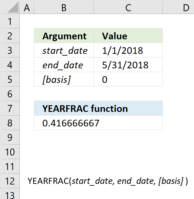
What is the YEARFRAC function?
The YEARFRAC function returns the fraction of the year based on the number of whole days between a start date and an end date. This is made possible because of how Excel handle dates.
What is an Excel date?
An Excel date is a serial number that Excel recognizes and can be filtered, sorted and used in other date calculations.
Excel dates are actually serial numbers formatted as dates, 1/1/1900 is 1 and 2/2/2018 is 43133. There are 43132 days between 2/2/2018 and 1/1/1900.
You can try this yourself, type 10000 in a cell, press CTRL + 1 and change the cell's formatting to date, press with left mouse button on OK. The cell now shows 5/18/1927.
What is a year?
A period of 365 days (366 days in leap years) based on the revolution of the Earth around the Sun. It represents one complete cycle of seasons - spring, summer, autumn, winter. Calendar years are numbered and divided into 12 months.
What is a leap year?
A leap year is a 366 day year occurring every 4 years to maintain calendar accuracy. A year containing an extra day, February 29th, that occurs once every 4 years.
The leap year was added to the Gregorian calendar to keep it aligned with the astronomical year. It occurs in years divisible by 4, except centurial years not divisible by 400.
What is a fraction?
A fraction has a numerator and a denominator:
- Numerator - The top number in a fraction.
- Denominator - The bottom number.
For example:
6/7
- The numerator is 6, meaning 6 parts.
- The denominator is 7, meaning the whole was split into 7 equal parts.
YEARFRAC function Syntax
YEARFRAC(start_date, end_date, [basis])
YEARFRAC function Arguments
| start_date | Required. |
| end_date | Required. |
| [basis] | Optional. Day count basis.
0 - Default value. US (NASD) 30/360 1 - Actual/actual 2 - Actual/360 3 - Actual/365 4 - European 30/360 |
YEARFRAC function example
Use the YEARFRAC function to calculate a part of a whole based on a date range relative to a year. This example demonstrates how to calculate the fraction of a year based on two specific dates located in cells C3 and C4 respectively. The [basis] argument is 0 (zero) in this example meaning it uses 30 days per month and a year has 360 days.
Formula in cell B8:
The YEARFRAC function in cell B8 returns 0.4166666 or 5/12 in fractions.
YEARFRAC function tips
Use the DATE function to create a date if you enter the date in the function.
Example:
The YEARFRAC function requires Excel dates to work properly, the DATE function allows you to create Excel dates by specifying the year, month, and day.
YEARFRAC function not working
If using the US (NASD) 30/360 basis which is argument 0 (zero), and the start_date argument is the last day in February the YEARFRAC function may return an incorrect result.
The YEARFRAC function may return an incorrect result if dates are entered as text values.
YEARFRAC returns
- the #VALUE! error value if start_date or end_date arguments are not valid dates.
- the #NUM! error value if basis < 0 or if basis > 4
Date and Time Functions – A to M 15 Mar 2024 4:22 AM (2 years ago)
Table of Contents
- How to use the DATE function
- How to use the DATEDIF function
- How to use the DATEVALUE function
- How to use the DAY function
- How to use the DAYS function
- How to use the EDATE function
- How to use the EOMONTH function
- How to use the HOUR function
- How to use the MINUTE function
- How to use the MONTH function
1. How to use the DATE function
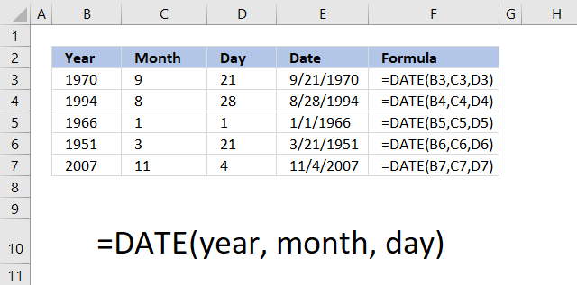
What is the DATE function?
The DATE function returns a number that acts as a date in the Excel environment.
Table of Contents
- Introduction
- Excel function syntax
- Function arguments
- DATE Function Example
- Add or subtract months and days
- Date function example
- What does the Date function do?
- Date function format
- Date function not working
- How to make Excel order by date
- Date function add days
- Date function subtract days
- Date function add months
- Last day of a given month
- Get Excel file
- Calculate date given weekday and week number (week starts on Sunday)
- Calculate date given weekday and week number (week starts on Monday)
1. Introduction
What is an Excel date?
Dates are stored numerically but formatted to display in human-readable date/time formats, this enables Excel to do work with dates in calculations.
For example, dates are stored as sequential serial numbers with 1 being January 1, 1900 by default. The integer part (whole number) represents the date the decimal part represents the time.
This allows dates to easily be formatted to display in many date/time formats like mm/dd/yyyy, dd/mm/yyyy and so on and still be part of calculations as long as the date is stored numerically in a cell.
You can try this yourself, type 10000 in a cell, press CTRL + 1 and change the cell's formatting to date, press with left mouse button on OK. The cell now shows 5/18/1927.
2. DATE Function Syntax
DATE(year, month, day)
3. DATE Function Arguments
| year | A number equal or higher than 1900. |
| month | A number between 1 (January) and 12 (December). You can use larger numbers as well. |
| day | A number between 1 and 31 based on the number of days in the month specified in argument month. |
4. DATE Function Example
The image above shows you the DATE function in column E. It uses three arguments, the first argument is the year found in column B.
The second argument is the month, shown in column C. Note that you need to use a number for the month.
The third argument is the day of the month, displayed in column D. Make sure you enter the correct day for the month, keep in mind most months have 30 days or 31 days. February has 28 days except for leap years that have 29 days.
5. Add or subtract months and days
If you use a month number larger than 12, for example 13, DATE(2009,13,1) the DATE function returns 1/1/2010. Month number zero returns the previous month.
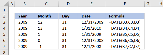
The same thing happens with a day number that is larger than 31 or smaller than 1.
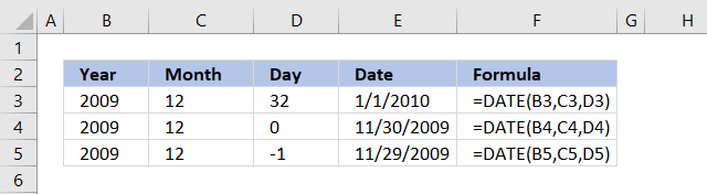
You can use that to do dynamic date series or do date-based calculations.
6. Date function example
The image above demonstrates the date function in column E, it uses values from column B, C and D.
Formula in cell F3:
7. What does the Date function do?
The DATE function returns an Excel date that you can use in formulas, Excel can't calculate dates in formulas unless you reference a cell containing an Excel date or create an Excel date using the DATE function.
Hardcoding dates in a formula are not possible, use the DATE function to create an Excel date.
Why is that?
Excel uses numbers formatted as dates, 1 is 1/1/1900, and 1/1/2000 is 36526.
Prove it?
Sure, type 1 in a cell and press Enter. Select the cell and press CTRL + 1 to format the cell.

A dialog box appears, select Date in Category: and press the "OK" button.

Number 1 is now formatted as an Excel date, the cell shows 1/1/1900.
8. Date function format

The animated image above shows you the "Format Cells" dialog box, it allows you to choose from many different date formatting types. Here is how:
- Select the cell.
- Press CTRL + 1 to open the "Format Cells" dialog box.
- Select Date in the Category:, see the image above.
- Pick a formatting type.
- Press with left mouse button on "OK" button to apply changes.

You can also use the TEXT function to format dates.
Formula in cell B2:
Explaining formula in cell B2
Step 1 - Create an Excel date
The DATE function calculates a serial number that represents a specific date based on three arguments. Year, month, and day.
DATE(year, month, day)
DATE(1900, 1, 1)
returns 1.
Step 2 - Return a number formatted as a date
The TEXT function formats a cell value based on given placeholder characters.
TEXT(value, format_text)
TEXT(DATE(1900, 1, 1), "d-m-yyyy")
becomes
TEXT(1, "d-m-yyyy")
and returns 1-1-1900.
9. Date function not working
- Did you spell the DATE function correctly?

Excel returns a #NAME? error if you didn't. - Check the arguments, they must be numerical. Text is not allowed.

Excel returns a #VALUE! error if any of the arguments contain a text value.
year - a number equal or larger than 0 (zero)
month - any number positive or negative
day - any number positive or negative - Did you use exactly three arguments?

Excel returns a dialog box: You've entered too many arguments for this function.
DATE(year, month, day) - Excel Date function returns the wrong date.

If you try a year before 1900 Excel returns a date that you probably didn't expect. Here is how Excel came up with that date. 1900+1800 = 1/1/3700 - The DATE function returns hashtags.

The DATE function can't return dates before 1/1/1900. The formula in cell B2 above tries to calculate an Excel date before 1/1/1900.
10. How to make Excel order by date

The image above shows a list of dates in column B, here is how to sort the dates.
- Press with right mouse button on any date in column B.
A popup menu appears.

- Press "Sort". Another popup menu appears.
- Press either "Sort Oldest to Newest" or "Sort Newest to Oldest".

Here is how to sort the dates using a formula.

Formula in cell D2:
Explaining formula in cell D2
Step 1 - Create a sequence of values from 1 to n
The ROWS function returns a number based on the number of rows in a cell reference.
ROWS(ref)
ROWS($A$1:A1)
returns 1.
Step 2 - Extract k-th largest serial number
The LARGE function calculates the k-th largest number.
LARGE(array, k)
LARGE($B$2:$B$17, ROWS($A$1:A1))
becomes
LARGE($B$2:$B$17, 1)
becomes
LARGE({45338; 53253; 49446; 51878; 48237; 52238; 44437; 53971; 49050; 47745; 45727; 45027; 49156; 49329; 48599; 49590}, 1)
and returns 53971 (10/6/2047) in cell D2.
11. Date function add days

The formula in cell C3 adds 10/25/2024 with 10 days specified in cell B3.
Formula in cell C3:
Explaining formula in cell C3
Step 1 - Add dates
The plus sign lets you add numbers in Excel formulas.
25+B3
becomes
25 + 10 equals 35.
Step 2 - Calculate serial number representing an Excel date
The DATE function calculates a serial number that represents a specific date based on three arguments. Year, month, and day.
DATE(year, month, day)
DATE(2024,10,25+B3)
becomes
DATE(2024,10,35)
and returns 45600 formatted as 11/4/2024 in cell C3.

12. Date function subtract days

The formula in cell C3 subtracts 10/25/2024 with 10 days specified in cell B3.
Formula in cell C3:
Explaining formula in cell C3
Step 1 - Subtract dates
The minus sign lets you subtract numbers in Excel formulas.
25-B3
becomes
25 - 10 equals 15.
Step 2 - Calculate serial number representing an Excel date
The DATE function calculates a serial number that represents a specific date based on three arguments. Year, month, and day.
DATE(year, month, day)
DATE(2024,10,25-B3)
becomes
DATE(2024,10,15)
and returns 45580 formatted as 11/4/2024 in cell C3.
13. Date function add months

The formula in cell E3 adds months based on the number in cell B3 to a date specified in cell C3.
Formula in cell C3:
Explaining formula in cell C3
Step 1 - Calculate year
The YEAR function returns a number representing the year based on an Excel date (serial number).
YEAR(serial_number)
YEAR(C3)
becomes
YEAR(1/14/2024)
becomes
YEAR(45305)
and returns 2024.
Step 2 - Calculate month
The MONTH function returns a number representing a month. 1 - January, ..., 12 - December.
MONTH(serial_number)
MONTH(C3)+B3
becomes
MONTH(45305)+10
becomes
1+10 equals 11.
Step 3 - Calculate day
The DAY function returns a number representing the day from an Excel date (serial number).
DAY(C3)
becomes
DAY(45305)
and returns 14.
Step 4 - Calculate date
The DATE function calculates a serial number that represents a specific date based on three arguments. Year, month, and day.
DATE(year, month, day)
DATE(YEAR(C3), MONTH(C3)+B3, DAY(C3))
becomes
DATE(2014, 11, 14)
and returns 45610 (11/14/2024).
14. Last day of a given month

The formula in cell D3 calculates the last day for a given month based on a date in cell B3. The date is 1/1/2024, the last day in January 2024 is 31.
The way this works is that the formula adds one month to the date in cell B3 then subtracts with 1 to get the last date of the previous month.
Formula in cell C3:
Explaining formula in cell C3
Step 1 - Calculate year
The YEAR function returns a number representing the year based on an Excel date (serial number).
YEAR(serial_number)
YEAR(B3)
becomes
YEAR(1/1/2024)
becomes
YEAR(45292)
and returns 2024.
Step 2 - Calculate month
The MONTH function returns a number representing a month. 1 - January, ..., 12 - December.
MONTH(serial_number)
MONTH(B3)+1
becomes
MONTH(45292)+1
becomes
1+1 equals 2.
Step 3 - Calculate day
The DAY function returns a number representing the day from an Excel date (serial number).
DAY(B3)
becomes
DAY(45292)
and returns 1.
Step 4 - Calculate the date
The DATE function calculates a serial number that represents a specific date based on three arguments. Year, month, and day.
DATE(year, month, day)
DATE(YEAR(B3),MONTH(B3)+1,1)-1
becomes
DATE(2014, 2, 1)-1
becomes
45323-1
and returns 45322 (1/31/2024).
15. Get Excel file
16. Calculate date given weekday and week number (week starts on Sunday)

This section demonstrates formulas that returns a date based on a week number and a weekday like Sun to Sat. It uses the current year to calculate the date.
La Thăng asks:
I want to find the day if given date and week, for example: if given Tuesday, 32nd week, 2015 >>> how to create a formula to point out 4/8/2015?

Formula in cell D6:
Explaining formula in cell D6
Step 1 - Calculate the first date of this year
The TODAY function returns today's date, the function is volatile meaning it recalculates every time you enter a value in a cell and press enter or press F9.
TODAY() returns 5/8/21.
Step 2 - Calculate the first date of this year
The YEAR function returns the year based on an Excel date.
YEAR(TODAY())
becomes
YEAR(44324)
and returns 2021.
Step 3 - Calculate the first date of this year
The DATE function returns an Excel date based on a year number, month number and day number.
DATE(year, month, day)
Year is a number from 1900 to 9999, month is a number from 1 to 12. 1 = January, ... , 12 = December. Day is usually a number between 1 and 31 but can be larger.
DATE(YEAR(TODAY()), 1, 1)
becomes
DATE(2021, 1, 1)
and returns 44197.
Step 4 - Subtract with the corresponding weekday number
The WEEKDAY function converts an Excel date to a number ranging from 1 to 7, based on when the week begins.
WEEKDAY(serial_number, [return_type])

If you live in the US the week in starts on Sundays, return_type is 1.
WEEKDAY(DATE(YEAR(TODAY()), 1, 1), 1)
becomes WEEKDAY(44197, 1)
and returns 6. 44197 is 1/1/2021 and that day is a Friday.
1 - Sunday, ... , 7 - Saturday.
Step 5 - Subtract date with weekday number
DATE(YEAR(TODAY()), 1, 1)-WEEKDAY(DATE(YEAR(TODAY()), 1, 1), 1)
becomes
44197 - 6 equals 44191.
Step 6 - Calculate and add the number of days from Monday/week 1 to Monday/(nth week -1)
+7*(D4-1)
Example, 7*(32-1)
becomes
7*31 and returns 217.
Step 7 - Calculate and add weekday number
The MATCH function returns the relative position of the given item in a cell range or array.
MATCH($D$4, {"Sun", "Mon", "Tue", "Wed", "Thu", "Fri", "Sat"}, 0)
If you week begins on sunday, this is the array you want to be using:
{"Sun", "Mon", "Tue", "Wed", "Thu", "Fri", "Sat"}.
Example, "Tue" returns 3. "Tue" is in position three in the array.
Step 8 - Add and subtract
44192+217+2 = 44411
44411 is 8/3/2021.
17. Calculate date given weekday and week number (week starts on Monday)

This example demonstrates a formula that works with weeks that begin with Mondays.
Formula in cell 5:
Note that the WEEKDAY function uses 2 in the second argument meaning the week begins with a Monday and the array in the second argument in the MATCH function begins with Monday.
Tip! You can shrink the formula if you can convert the weekday to a number yourself.
2. How to use the DATEDIF function
What is the DATEDIF function?
The DATEDIF function returns the number of days, or months, or years between two dates. The DATEDIF function exists in order to ensure compatibility with Louts 1-2-3.
DATEDIF function not found?

You may think that the DATEDIF function is not in Excel when you type the function in the formula bar. The DATEDIF function is not missing, however, it doesn't show up in the list.
Type the DATEDIF function, the beginning parentheses, the arguments, the closing parentheses, and it will work.

What are dates in Excel?
Dates are stored numerically but formatted to display in human-readable date/time formats, this enables Excel to do work with dates in calculations.
For example, dates are stored as sequential serial numbers with 1 being January 1, 1900 by default. The integer part (whole number) represents the date the decimal part represents the time.
This allows dates to easily be formatted to display in many date/time formats like mm/dd/yyyy, dd/mm/yyyy and so on and still be part of calculations as long as the date is stored numerically in a cell.
Table of Contents
1. DATEDIF function Syntax
DATEDIF(start_date,end_date,unit)
Note, this function shows no arguments in the formula bar.
2. DATEDIF function Arguments
| start_date | Required. The beginning date of the range you want to calculate. |
| end_date | Required. The ending date of the period. |
| unit | Required. This determines what the function returns. See table below. |
Unit argument
| Unit | Output |
| "Y" | Complete years in the range. |
| "M" | Complete months in the range. |
| "D" | Days in the range. |
| "MD" | Months and years of the dates are ignored. Don't use this argument, may return incorrect results. |
| "YM" | Returns months. Days and years of the date arguments are ignored. |
| "YD" | Returns days. The years of the date arguments are ignored. |
3. DATEDIF example - calculate complete years between two dates
This example demonstrates how to calculate complete years between two given dates using the DATEDIF function. The first date is specified in cell B3 and the second date in cell C3.
Formula in cell D3:
The third argument determines the unit to calculate, in this case, it is "Y" which stands for year. Excel returns 2 in cell D3 meaning there are two complete years between "1/4/2013" and "1/6/2015".
4. DATEDIF example - calculate days between two dates
This example shows how to calculate days between two given dates using the DATEDIF function. The first date is specified in cell B4 and the second date in cell C4.
Formula in cell D4:
The third argument determines the unit to calculate, in this case, it is "D" which stands for day. Excel returns 582 in cell D4 meaning there are 582 days between "11/20/2010" and "6/24/2012".
There is an easier way to calculate days between two dates in Excel, simply subtract the dates.
Formula in cell D4:
For example,
the first date is 1/1/2030 and the second date is 1/2/2030, both calculations return 1 day, however, you may think it is two days between the dates. This is because if you calculate the end date inclusive or not.
If you want to calculate the end date also included then use this:
Formula in cell D4:
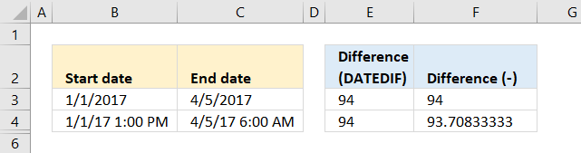
The picture above shows you this issue in cell E4.
A much easier formula is to simply subtract the earlier date from the later date. Excel dates are actually numbers between 1 and 99999 formatted as dates, this allows you to do mathematical operations to dates.
You can see that yourself by selecting a cell containing a date and then press CTRL + 1. This opens a dialog box where you can see how the cell is formatted.
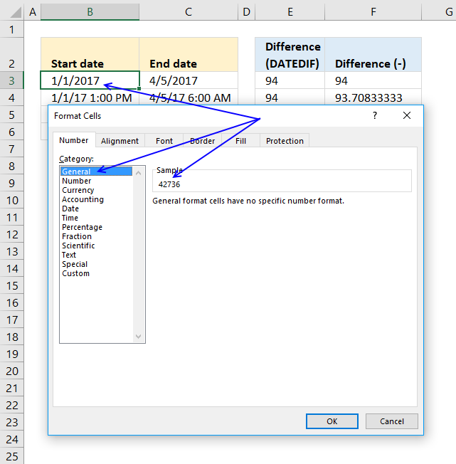
Press with mouse on General to show the number. 1/1/2017 is in fact 42736. Number 1 is 1/1/1900.
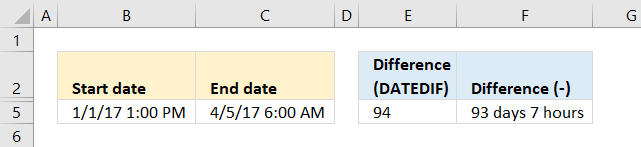
If you use dates and time and want to calculate the number of days and hours between two dates use the following formula:
The result is displayed in cell F5 on the picture above.
INT(C5-B5)& " days "
The INT function removes the decimal part from the number returning complete days. The & (ampersand) concatenates the number with the text string " days".
HOUR(B5-C5-INT(B5-C5))&" hours"
The HOUR function returns a number representing the hour. The decimal part of the number is the time, in this case, hours. To get the decimal part simply subtract the integer part from the number, this is where the INT function comes in.
Lastly, the ampersand & character concatenates the hour number with " hours". You can get even greater detail by using the MINUTE and SECOND functions as well.
Get Excel *.xlsx
5. Calculate days between two dates ignoring the years
This example demonstrates how to calculate days between two given dates ignoring the years using the DATEDIF function. The first date is specified in cell B3 and the second date in cell C3.
Formula in cell D5:
The third argument determines the unit to calculate, in this case, it is "YD" which stands for days ignoring years. Excel returns 276 in cell D5 meaning there are 276 days between November 20th and June 24th.
6. Calculate complete months between two dates
This example displays how to calculate complete months between two given dates using the DATEDIF function. The first date is specified in cell B6 and the second date in cell C6.
Formula in cell D6:
The third argument determines the unit to calculate, in this case, it is "M" which stands for complete months. Excel returns 14 in cell D6 meaning there are 14 complete months between "8/15/2013" and "10/27/2014".
7. DATEDIF function not working
Don't use the "MD" argument, it may return incorrect results.
Make sure Excel recognizes the date as an Excel date. If the date is interpreted as a text value no calculations can be done.
3. How to use the DATEVALUE function

What is the DATEVALUE function?
The DATEVALUE function returns an Excel date value (serial number) based on a date stored as text.
Table of Contents
1. Introduction
What are dates in Excel?
Dates are stored numerically but formatted to display in human-readable date/time formats, this enables Excel to do work with dates in calculations.
For example, dates are stored as sequential serial numbers with 1 being January 1, 1900 by default. The integer part (whole number) represents the date the decimal part represents the time.
This allows dates to easily be formatted to display in many date/time formats like mm/dd/yyyy, dd/mm/yyyy and so on and still be part of calculations as long as the date is stored numerically in a cell.
You can try this yourself, type 10000 in a cell, press CTRL + 1 and change the cell's formatting to date, press with left mouse button on OK. The cell now shows 5/18/1927.
Why are dates stored as text in Excel?
Dates are not stored as text in Excel they are stored as numbers, however, Excel tries to identify values as text, numbers, Boolean values, dates, and time automatically but may fail in rare occasions.
This may happen when you import data from the internet, databases, text files, and other sources. You can convert the dates to Excel dates if you like but it can be a tedious and time consuming task.
The DATEVALUE function lets you convert the text date in the formula to an Excel date without you first converting them on the worksheet.
How to enter valid dates in Excel?

Valid dates are right-aligned in a cell just like numbers, invalid dates are identified as text values and left-aligned. The image above shows that / (forward slash) and - (dash) are valid delimiting characters in Excel dates, demonstrated in cells B2 and B3.
A dot and no delimiters at all, shown in cells B4 and B5, are invalid, these dates are left-aligned by Excel. The DATEVALUE cant properly identify these date values either, you need to change these dates by hand or using the methods described below.
2. DATEVALUE function Syntax
DATEVALUE(date_text)
3. DATEVALUE function Arguments
| date_text | Required. The date stored as text you want to convert to an Excel date (serial number). |
4. DATEVALUE function example
A date stored as text can't be sorted, filtered or be used in Excel date calculations. You need to convert the date stored as text to a date that Excel recognizes. The image above shows dates stored as text in cell range B3:B7.
Formula in cell C3:
Explaining formula
DATEVALUE(B3)
becomes
DATEVALUE("1/4/2013")
and returns
41278 which is the corresponding serial number Excel uses for the date "1/4/2013".
5. DATEVALUE function not working
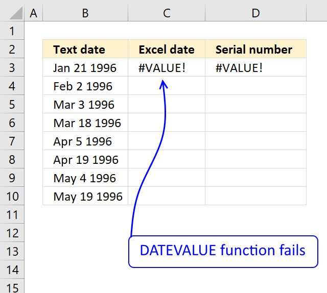
The DATEVALUE function returns an Excel date value (serial number) based on a date stored as text. However, it must be a valid text date which is determined by your date and time settings (national settings) on your operating system.
Formula in cell C3:
5.1. Verify your date and time settings

Microsoft recommends that you verify your date and time settings so they are compatible with the text date format. On a "Windows 10" operating system open the Control Panel and then "National Settings" and see if you can find a supported date setting. Both the short and long dates must match.
5.2. Convert a text date to an Excel date using a formula
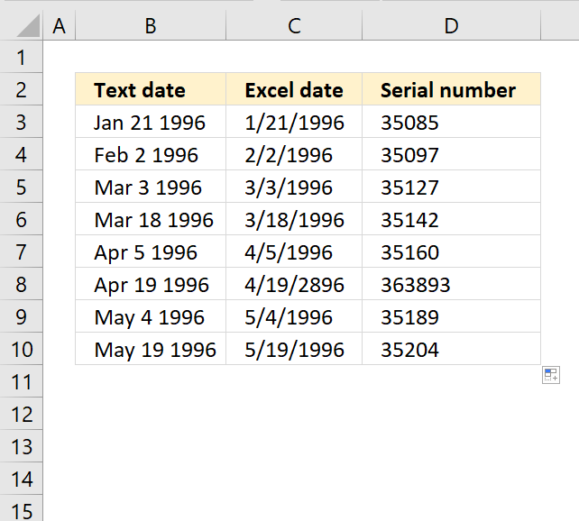
I could not find a setting that worked with the text date above so I created the following formula in cell C3.
The picture above shows the output of the formula in column C.
5.2.3. Explaining the formula in cell C3
Step 1 - Extract year from string
To extract the year from the text date in cell B3 I simply use the RIGHT function to extract the 4 last characters.
The RIGHT function extracts a specific number of characters always starting from the right.
RIGHT(text,[num_chars])
RIGHT(B3, 4)
becomes
RIGHT("Jan 21 1996", 4)
and returns 1996.
Step 2 - Extract month abbreviation from string
The month number is a little harder since it is built of three letters. To get the three letters from B3 I use the LEFT function.
The LEFT function extracts a specific number of characters always starting from the left.
LEFT(text, [num_chars])
LEFT(B3, 3)
becomes
LEFT("Jan 21 1996", 3)
and returns "Jan".
Step 3 - Convert month to a number
The MATCH function returns the relative position of an item in an array or cell reference that matches a specified value in a specific order.
MATCH(lookup_value, lookup_array, [match_type])
MATCH(LEFT(B3, 3), {"Jan"; "Feb"; "Mar"; "Apr"; "May"; "Jun"; "Jul"; "Aug"; "Sep"; "Oct"; "Nov"; "Dec"}, 0)
becomes
MATCH("Jan", {"Jan"; "Feb"; "Mar"; "Apr"; "May"; "Jun"; "Jul"; "Aug"; "Sep"; "Oct"; "Nov"; "Dec"}, 0)
and returns 1. "Jan" is the first value in the array.
Step 4 - Extract day from string
The MID function returns a substring from a string based on the starting position and the number of characters you want to extract.
MID(text, start_num, num_chars)
MID(B3, 4, 3)
becomes
MID("Jan 21 1996", 4, 3)
and returns " 21".
Step 5 - Create an Excel date
The DATE function allows you to create an Excel date based on a year, month, and day number.
The arguments are DATE(year, month, day).
DATE(RIGHT(B3, 4), MATCH(LEFT(B3, 3), {"Jan"; "Feb"; "Mar"; "Apr"; "May"; "Jun"; "Jul"; "Aug"; "Sep"; "Oct"; "Nov"; "Dec"}, 0), MID(B3, 4, 3))
becomes
DATE(1996, 1, 21)
and returns 1/21/1996 in cell C3.
Get Excel *.xlsx file
DATEVALUE function not working.xlsx
5.3 Example

This example shows that the DATEVALUE function can't handle a date with a dot as a delimiting character.
Formula in cell D3:
The DATEVALUE function returns a #VALUE! error.
How to create an Excel date from dates using dots as delimiting characters?
The SUBSTITUTE function lets you replace a given text string with a new text string.
Formula in cell D3 that works:
Explaining formula
Step 1 - Substitute dots with forward slash
The SUBSTITUTE function replaces a specific text string in a value. Case sensitive.
Function syntax: SUBSTITUTE(text, old_text, new_text, [instance_num])
SUBSTITUTE(B3,".","/")
becomes
SUBSTITUTE("1.4.2013",".","/")
and returns
"1/4/2013".
Step 2 - Convert text date to an Excel date
The DATEVALUE function returns an Excel date value (serial number) based on a date stored as text.
Function syntax: DATEVALUE(date_text)
DATEVALUE(SUBSTITUTE(B3,".","/"))
becomes
DATEVALUE("1/4/2013")
and returns 41278. Here is how to format the cell value as a date:
- Select the cell (D3).
- Press CTRL + 1 to open the "Format Cells.." dialog box.

- Select category : Date
- Pick a date formatting.
- Press with mouse on the "OK" button.

This example shows that the DATEVALUE function can't handle a date without delimiting characters.
Formula in cell D3:
The DATEVALUE function returns a #VALUE! error.
How to create an Excel date from dates without delimiting characters?
Formula in cell D3 that works:
Explaining formula
Step 1 - Extract year from date
The RIGHT function extracts a specific number of characters always starting from the right.
Function syntax: RIGHT(text,[num_chars])
RIGHT(B3,4)
becomes
RIGHT("01042013",4)
and returns "2013".
Step 2 - Extract month from date
The LEFT function extracts a specific number of characters always starting from the left.
Function syntax: LEFT(text, [num_chars])
LEFT(B3,2)
becomes
LEFT("01042013",2)
and returns "01".
Step 3 - Extract day from date
The MID function returns a substring from a string based on the starting position and the number of characters you want to extract.
Function syntax: MID(text, start_num, num_chars)
MID(B3,3,2)
becomes
MID("01042013",3,2)
and returns "04".
Step 4 - Convert to an Excel date
The DATE function returns a number that acts as a date in the Excel environment.
Function syntax: DATE(year, month, day)
DATE(RIGHT(B3,4),LEFT(B3,2),MID(B3,3,2))
becomes
DATE("2013","01","04")
and returns 41278.
4. How to use the DAY function
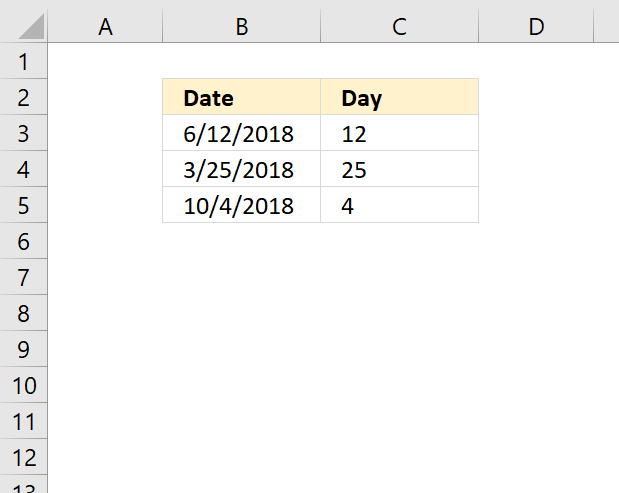
What is the DAY function?
The DAY function extracts the day as a number from an Excel date.
Table of Contents
1. DAY Function Syntax
DAY(serial_number)
2. DAY Function Arguments
| serial_number | Required. The Excel date value you want to extract the day number from. |
Excel dates are actually numbers formatted as dates. January 1, 1900 is serial number 1, and January 1, 2008 is serial number 39448 because it is 39,448 days after January 1, 1900.
3. DAY function example
The image above demonstrates a formula in cell C3 that extracts the day number from a date, however, the date must be an Excel date.
Formula in cell C3:
To understand the DAY function I need to explain that it needs an Excel date in order to calculate the day properly. The date in cell B3 is an Excel date meaning it is a number formatted as a date. 1 is 1/1/1900 and 1/1/2000 is 36526 meaning there are 36526 days between the dates.
You can verify this, select a cell containing 1/1/2000 and press CTRL + 1 to open the "Format Cells" dialog box.

4. DAY function not working
- Check your spelling.
- Make sure the date is an Excel date.
How do I know the date is recognized as an Excel date?
Check the "Format Cells" dialog box and press with left mouse button on category "General". You should see a number and not a date.
How do I convert a date to an Excel date?
Try using the DATEVALUE function to convert a text date to an Excel date. Read this article if it is not working.
5.1 DAY function alternative - TEXT function

Formula in cell C3:
5.1.1 Explaining formula
Step 1 - TEXT function
The TEXT function lets you format values.
TEXT(value, format_text)
value - The string you want to format. You can use a cell reference here or use a text string.
format_text - Formatting code allowing you to change the way, for example, a date or a number is displayed to the Excel user.
Step 2 - Populate arguments
The TEXT function has two arguments.
value - B3
format_text - "d"
"d" is an abbreviation for day. A single "d" returns the day like this: 1. A double "dd" returns 01.
Check out this article to learn more about formatting codes in the TEXT function.
Step 3 - Evaluate TEXT function
TEXT(B3, "d")
becomes
TEXT(43263, "d")
and returns 12.
5.2 DAY function alternative - Cell formatting

You can also show the day number using cell formatting, the image above shows cell formatting applied to cell C5.
How to apply cell formatting:
- Select cell C3.
- Press CTRL + 1 to open the "Format Cells" dialog box.
- Press with left mouse button on "Category" Custom, see the image above.
- Enter d below Type:
- Press with left mouse button on the OK button to apply changes.
6. Filter dates based on a given day number

Formula in cell D3:
Explaining formula
Step 1 - Calculate day number for each date value
DAY(B3:B11)
becomes
DAY({44667; 44667; 44700; 44707; 45006; 45051; 45054; 45075; 45079})
and returns
{16; 15; 16; 26; 16; 16; 8; 29; 16}.
Step 2 - Compare month number to condition
The equal sign lets you check if values are equal, note that this does not perform a case-sensitive comparison. Check out the EXACT function if upper and lower letters matter.
DAY(B3:B11)=16
becomes
{16; 15; 16; 26; 16; 16; 8; 29; 16}=16
and returns
{TRUE; FALSE; TRUE; FALSE; TRUE; TRUE; FALSE; FALSE; TRUE}.
Step 3 - Extract dates meeting the condition
The FILTER function is a new function available to Excel 365 subscribers. It lets you extract values based on a condition or criteria.
FILTER(array, include, [if_empty])
FILTER(B3:B11, DAY(B3:B11)=16)
becomes
FILTER({44667; 44667; 44700; 44707; 45006; 45051; 45054; 45075; 45079}, {TRUE; FALSE; TRUE; FALSE; TRUE; TRUE; FALSE; FALSE; TRUE})
and returns
{44667; 44700; 45006; 45051; 45079}.
7. Create a dynamic calendar using the DAY function

The formula in cell B4 is a dynamic array formula and works only in Excel 365. The SEQUENCE function is only available to Excel 365 subscribers.
The formula uses the provided date in cell B2 to calculate all dates for that month. Make sure you only use Excel dates in cell B2 and that the date is the first date in any given month.
The dates in B4:H9 automatically refresh as soon as a new date is entered in cell B2, this is why it is called a dynamic calendar.
Excel 365 formula in cell B4:
Explaining formula
The dynamic array formula in cell B4 is entered as a regular formula, however, it spills values to the right and below as far as needed.
Make sure the adjacent cells are empty or a #SPILL! error is shown.
Step 1 - Calculate weekday
This step is needed in order to calculate the first date in the week, it is most often not the same date as the first date in a month. It is the 27th in this example, shown in the image above.
The WEEKDAY function returns a number representing the weekday in a week. 1 - Sunday, 2 - Monday, and so on.
WEEKDAY(serial_number,[return_type])
WEEKDAY(B2,1)
becomes
WEEKDAY(44621, 1)
and returns 3. This means that March the 1st, 2022 is a Tuesday.
Step 2 - Create an array large enough to populate a monthly calendar
The SEQUENCE function creates a list of sequential numbers to a cell range or array. It is located in the Math and trigonometry category and is only available to Excel 365 subscribers.
SEQUENCE(rows, [columns], [start], [step])
SEQUENCE(6,7)
returns
{1, 2, 3, 4, 5, 6, 7; 8, 9, 10, 11, 12, 13, 14; 15, 16, 17, 18, 19, 20, 21; 22, 23, 24, 25, 26, 27, 28; 29, 30, 31, 32, 33, 34, 35; 36, 37, 38, 39, 40, 41, 42}.
Note the delimiting characters used in the array above, the comma separates values between columns and the semicolon between rows. Your setup may use other delimiting characters, you can change these in the regional settings.
Step 3 - Calculate the date for the first sunday
This is often a date in the previous month. The plus and minus sign lets you perform arithmetic calculations in an Excel formula.
B2-WEEKDAY(B2,1)+SEQUENCE(6,7)
becomes
44621 - 3 + {1, 2, 3, 4, 5, 6, 7; 8, 9, 10, 11, 12, 13, 14; 15, 16, 17, 18, 19, 20, 21; 22, 23, 24, 25, 26, 27, 28; 29, 30, 31, 32, 33, 34, 35; 36, 37, 38, 39, 40, 41, 42}
and returns
{44619, 44620, 44621, 44622, 44623, 44624, 44625; 44626, 44627, 44628, 44629, 44630, 44631, 44632; 44633, 44634, 44635, 44636, 44637, 44638, 44639; 44640, 44641, 44642, 44643, 44644, 44645, 44646; 44647, 44648, 44649, 44650, 44651, 44652, 44653; 44654, 44655, 44656, 44657, 44658, 44659, 44660}
Step 4 - Calculate the day for each date in the array
DAY(B2-WEEKDAY(B2,1)+SEQUENCE(6,7))
becomes
DAY({44619, 44620, 44621, 44622, 44623, 44624, 44625; 44626, 44627, 44628, 44629, 44630, 44631, 44632; 44633, 44634, 44635, 44636, 44637, 44638, 44639; 44640, 44641, 44642, 44643, 44644, 44645, 44646; 44647, 44648, 44649, 44650, 44651, 44652, 44653; 44654, 44655, 44656, 44657, 44658, 44659, 44660})
and returns
{27, 28, 1, 2, 3, 4, 5; 6, 7, 8, 9, 10, 11, 12; 13, 14, 15, 16, 17, 18, 19; 20, 21, 22, 23, 24, 25, 26; 27, 28, 29, 30, 31, 1, 2; 3, 4, 5, 6, 7, 8, 9}.
5. How to use the DAYS function
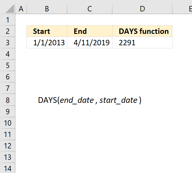
What is the DAYS function?
The DAYS function calculates an integer that represents the number of days between two dates.
There is, actually, an easier way to calculate the number of days between two dates. Simply subtract C3 by B3 like this: = C3-B3 and you will get the number of days.
The DATEDIF function is also able to calculate the number of days between two dates.
What are dates in Excel?
Dates are stored numerically but formatted to display in human-readable date/time formats, this enables Excel to do work with dates in calculations.
For example, dates are stored as sequential serial numbers with 1 being January 1, 1900 by default. The integer part (whole number) represents the date the decimal part represents the time.
This allows dates to easily be formatted to display in many date/time formats like mm/dd/yyyy, dd/mm/yyyy and so on and still be part of calculations as long as the date is stored numerically in a cell.
You can try this yourself, type 10000 in a cell, press CTRL + 1 and change the cell's formatting to date, press with left mouse button on OK. The cell now shows 5/18/1927.
Related functions
| Excel Function | Description |
|---|---|
| DAY(date) | Returns the day of the month (1-31) |
| DAYS(end_date, start_date) | Returns the number of days between two dates |
| NETWORKDAYS(start_date, end_date) | Returns the number of workdays between two dates |
| DATEDIF(start_date, end_date, unit) | Returns the time between two dates in specified units like years, monts, etc |
| EDATE(start_date, months) | Returns the date that is the indicated number of months before or after start_date |
| EOMONTH(start_date, months) | Returns the last day of the month before or after start_date by months |
| NETWORKDAYS.INTL(start_date, end_date, weekend) | Returns workdays between dates with custom weekend parameters |
| WORKDAY(start_date, days) | Returns a date days away from the start_date, skipping weekends |
DAYS function Syntax
DAYS(end_date, start_date)
DAYS function Arguments
| end_date | Required. The end date of the date range you want to calculate. |
| start_date | Required. The start date of the date range you want to calculate. |
DAYS function example

This example shows the DAYS function in cell D3, in the image above, calculating the difference in days between the specified cells C3 and B3.
Formula in cell D3:
The DAYS function calculates 1 day between 1/1/2030 and 1/2/2030. Why, you may wonder? There are two days in that date range? It depends how you calculate. 1/1/2030 is 47484 and 1/2/2030 is 47485. 47485 - 47484 equals 1.
This is because if you calculate the end date inclusive or not. If you want to include the end date in the calculation then use this:
Formula in cell D3:
DAYS function tips and tricks
Why are dates sometimes stored as text in Excel?

Excel tries to identify values as text, numbers, Boolean values, dates, and time automatically but may fail in rare occasions. This may happen when you import data from the internet, databases, text files, and other sources. You can convert the dates to Excel dates if you like but it can be a tedious and time consuming task.
There is no need to convert text dates to Excel dates, the DAYS function handles text dates properly.
DAYS function not working

The image above shows two dates containing a dot as a delimiting character, this makes Excel return an error.
The DAYS function returns #VALUE! error if a date is not recognized, here is a formula to fix this problem: DATEVALUE function
6. How to use the EDATE function
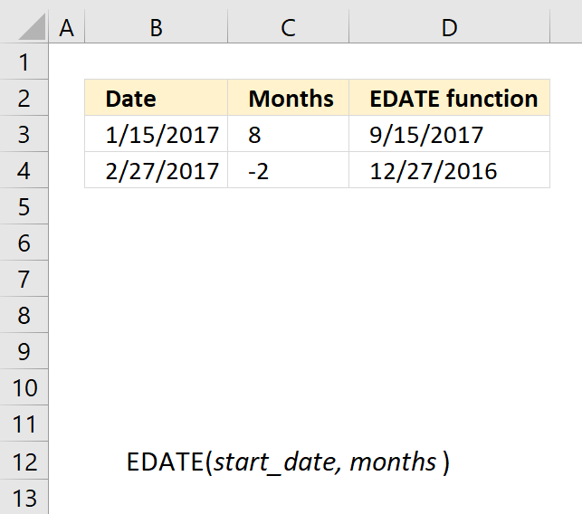
What is the EDATE function?
The EDATE function returns a date determined by a start date and a number representing the months. Use EDATE to calculate maturity dates or due dates that fall on the same day of the month as the date of issue.
What are dates in Excel?
Dates are stored numerically but formatted to display in human-readable date/time formats, this enables Excel to do work with dates in calculations.
For example, dates are stored as sequential serial numbers with 1 being January 1, 1900 by default. The integer part (whole number) represents the date the decimal part represents the time.
This allows dates to easily be formatted to display in many date/time formats like mm/dd/yyyy, dd/mm/yyyy and so on and still be part of calculations as long as the date is stored numerically in a cell.
You can try this yourself, type 10000 in a cell, press CTRL + 1 and change the cell's formatting to date, press with left mouse button on OK. The cell now shows 5/18/1927.
What is a maturity date?
The maturity date is the date on which the principal amount of a security becomes due and payable to the holder. It applies to fixed-income securities like bonds, notes, bills where the issuer must repay the principal on the maturity date.
At maturity, the debt is fully repaid. The security might cease to exist after maturity. Maturity dates affect interest rate risk - longer terms have higher risk. The final coupon payment is made on the maturity date.
What is a due date?
The due date is the date on which a debt payment is due to be paid by a borrower to a lender. It applies to loans, mortgages, credit cards, accounts receivables where periodic payments are required.
A due date recurrence can be monthly, quarterly, annually based on the terms. Missing a due date can result in late fees or interest charges.
Related functions
| Excel Function | Description |
|---|---|
| DATEDIF(start_date, end_date, unit) | Returns the time between two dates in specified units like complete years or months |
| EDATE(start_date, months) | Returns the date that is the indicated number of months before or after start_date |
| EOMONTH(start_date, months) | Returns the last day of the month before or after start_date by months |
| MONTH(date) | Returns the month of a date (1-12) |
| DATE(year, month, day) | Returns an Excel date |
EDATE function Syntax
EDATE(start_date, months)
EDATE function Arguments
| start_date | Required. A start date. |
| months | Required. The number of months before or after start_date. You are allowed to use negative numbers here. A negative number makes the function return an earlier date than the start date. |
The first argument is an Excel date, make sure it is not invalid. The second argument is an integer, negative values are also possible.
EDATE function example

The image above demonstrates the EDATE function in cells D3 and D4, the start dates are specified in cells B3 and B4. The number of months are in cells C3 and C4.
Formula in cell D3:
The first date in cell B3 is "1/15/2017", the number of months in cell C3 and the result in cell D3 is "9/15/2017" which is exactly 8 months later.
Calculate quarterly dates

This example demonstrates how to calculate four different dates in the same calculation using arrays in Excel. The calculated dates are exactly three months a part from the start date.
Dynamic array formula in cell D3:
{3;6;9;12} is an array of numbers separated by a semicolon. Excel performs four different calculations in the same cell and returns an array to cell D3 and the cells below as far as needed. This is called spilling and is a new feature in Excel 365.
Calculate bi-monthly dates

This example demonstrates how to calculate six different dates in the same calculation using arrays in Excel. The calculated dates are exactly two months a part from the start date.
Dynamic array formula in cell D3:
Explaining formula in cell D3
Step 1 - Create a sequence from 2 to 12 with step 2
The SEQUENCE function creates a list of sequential numbers.
Function syntax: SEQUENCE(rows, [columns], [start], [step])
SEQUENCE(6,,2,2)
returns
{2;4;6;8;10;12}
Step 2 - Calculate dates
EDATE(B3,SEQUENCE(6,,2,2))
becomes
EDATE(B3,{2;4;6;8;10;12})
and returns
{42809;42870;42931;42993;43054;43115}.
EDATE function tips and tricks

Use a negative number as the month argument to get a date before the start date. The image above shows the start date in cell B3, -2 in cell C3 which represents the month argument and the result in cell D3.
2/27/2030 minus two months is 12/27/2029
EDATE function not working

An invalid date demonstrated in cell B5 returns a #VALUE! error displayed in cell D5. Use the method explain here to convert invalid dates to dates that work: DATEVALUE function
The EDATE function truncates a decimal value representing months argument, shown in cell C3 and D3.
What is truncate?
Removing the decimal leaving only the whole number. For example, truncate 7.9 and you get 7.
EDATE function alternative
The DATE function creates an Excel date based on three arguments: year, month, and day. It can be used to calculate a date for a given number of months in the future, or in the past, just like the EDATE function.
- year - a number containing four digits equal to or larger than 1900.
- month - a number between 1 and 12 representing the months in a year: January to December.
- a - variable representing the months argument in the EDATE function.
- day - a number representing the day of the date from 1 to 31.
7. How to use the EOMONTH function
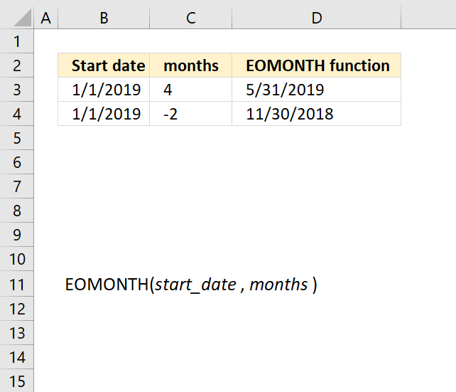
What is the EOMONTH function?
The EOMONTH function returns an Excel date for the last day of a given month using a number and a start date. Use EOMONTH to calculate maturity dates or due dates that fall on the last day of the month.
What is EOMONTH an abbreviation of?
EOMONTH stand for End Of month.
What are dates in Excel?
Dates are stored numerically but formatted to display in human-readable date/time formats, this enables Excel to do work with dates in calculations.
For example, dates are stored as sequential serial numbers with 1 being January 1, 1900 by default. The integer part (whole number) represents the date the decimal part represents the time.
This allows dates to easily be formatted to display in many date/time formats like mm/dd/yyyy, dd/mm/yyyy and so on and still be part of calculations as long as the date is stored numerically in a cell.
You can try this yourself, type 10000 in a cell, press CTRL + 1 and change the cell's formatting to date, press with left mouse button on OK. The cell now shows 5/18/1927.
What is a maturity date?
The maturity date is the date on which the principal amount of a security becomes due and payable to the holder. It applies to fixed-income securities like bonds, notes, bills where the issuer must repay the principal on the maturity date.
At maturity, the debt is fully repaid. The security might cease to exist after maturity. Maturity dates affect interest rate risk - longer terms have higher risk. The final coupon payment is made on the maturity date.
What is a due date?
The due date is the date on which a debt payment is due to be paid by a borrower to a lender. It applies to loans, mortgages, credit cards, accounts receivables where periodic payments are required.
A due date recurrence can be monthly, quarterly, annually based on the terms. Missing a due date can result in late fees or interest charges.
Related functions
| Excel Function | Description |
|---|---|
| DATEDIF(start_date, end_date, unit) | Returns the time between two dates in specified units like complete years or months |
| EDATE(start_date, months) | Returns the date that is the indicated number of months before or after start_date |
| EOMONTH(start_date, months) | Returns the last day of the month before or after start_date by months |
| MONTH(date) | Returns the month of a date (1-12) |
| DATE(year, month, day) | Returns an Excel date |
EOMONTH function Syntax
EOMONTH(start_date, months)
EOMONTH function Arguments
| start_date | Required. A date that represents the starting date. Don't use text dates, use Excel dates, see comments below. |
| months | Required. A number that determines how many months before or after the start date. A negative value returns a date earlier than the start_date. |
EOMONTH function example

The image above shows the EOMONTH function cell D3 calculating the last day of the month based on a start date specified in cell B3 and the number of months specified in cell C3.
Formula in cell D3:
The function calculates 5/31/2030 based on the start date 1/1/2030 and add 4 months to that. The last day in May 2030 is 31.
Calculate quarterly dates for the last day of a given month

This example demonstrates how to calculate four different dates in the same calculation using arrays in Excel. The calculated dates are exactly three months a part from the start date and is the last date in that particular month.
Formula in cell D3:
{3;6;9;12} is an array of numbers separated by a semicolon. Excel performs four different calculations in the same cell and returns an array to cell D3 and the cells below as far as needed. This is called spilling and is a new feature in Excel 365.
Calculate bi monthly dates for the last day of a given month

This example demonstrates how to calculate six different dates in the same calculation using arrays in Excel. The calculated dates are exactly two months a part from the start date and is the last date in that particular month.
Formula in cell D3:
Explaining formula in cell D3
Step 1 - Create a sequence from 2 to 12 with step 2
The SEQUENCE function creates a list of sequential numbers.
Function syntax: SEQUENCE(rows, [columns], [start], [step])
SEQUENCE(6,,2,2)
returns
{2;4;6;8;10;12}
Step 2 - Calculate dates
EOMONTH(B3,SEQUENCE(6,,2,2))
becomes
EOMONTH(B3,{2;4;6;8;10;12})
and returns
{49399;49460;49521;49582;49643;49705}.
EOMONTH function tips

Use a negative number as the month argument to get a date before the start date. The image above shows the start date in cell B3, -2 in cell C3 which represents the month argument and the result in cell D3.
1/1/2035 minus two months is November 2034 and the last date in that month is 11/30/2034.
EOMONTH function not working

An invalid date demonstrated in cell B5 returns a #VALUE! error displayed in cell D5. Use the method explain here to convert invalid dates to dates that work: DATEVALUE function
The EOMONTH function truncates a decimal value representing the months argument.
What is truncate?
Removing the decimal leaving only the whole number. For example, truncate 7.9 and you get 7.
EOMONTH function alternative

Formula in cell D3:
Explaining formula in cell D3
Step 1 - Calculate the year
The YEAR function converts a date to a number representing the year in the date.
Function syntax: YEAR(serial_number)
YEAR(B3)
becomes
YEAR(49310)
and returns "2035".
Step 2 - Calculate the month
The MONTH function extracts the month as a number from an Excel date.
Function syntax: MONTH(serial_number)
MONTH(B3) +C3 + 1
becomes
MONTH(49310) + 4 + 1
becomes
1 + 4 + 1
and returns 6.
Step 3 - Calculate the Excel date
The DATE function returns a number that acts as a date in the Excel environment.
Function syntax: DATE(year, month, day)
DATE(YEAR(B3),MONTH(B3)+C3+1,1)
becomes
DATE(2035,6,1)
and returns "6/1/2035" (49460)
Step 4 - Subtract Excel date by 1
DATE(YEAR(B3),MONTH(B3)+C3+1,1) - 1
becomes
49460 - 1
and returns
49459 (5/31/2035)
8. How to use the HOUR function

What is the HOUR function?
The HOUR function returns an integer representing the hour of an Excel time value. The returning number is ranging from 0 (12:00 A.M.) to 23 (11:00 P.M.).
Table of Contents
1. What is an integer?
An integer is a whole number that can be positive, negative, or zero, but not a fraction or decimal. Excel can't calculate the hour based on negative integers.
What is an Excel time value?
Excel time is actually a decimal number ranging between 0 and 1 in Excel and then formatted as time.
For example, 12:00 PM is represented as 0.5 because it is half of a day, you can verify this by typing 12:00 PM in a cell and then change the cell formatting to general. This will show the value as Excel interprets it.
How does Excel recognize time values?
Excel recognizes certain text strings like "6:45 PM" as valid time values. A recognized time value is right aligned in the cell just like a regular number, shown in the image below in cell B2.
A time number that is not recognized is left aligned which is demonstrated in cell B4 in the image above. This visual feedback lets you easily spot values that need closer inspection.
What is an hour in an Excel time value?

1/24 or approx. 0.04166667 represents one hour in Excel time value. Excel uses a number 0 <= x <= 1 in decimal form to represent time in a worksheet. 0 is zero hours and 1 is 24 hours. To get one hour we must divide 1 by 24 and we get 1/24.
Why is 1 equal to 24 hours?
This has to do how Excel handles dates. Each date is represented by an integer and one day is 1 in Excel.
Dates are stored numerically but formatted to display in human-readable date/time formats, this enables Excel to do work with dates in calculations.
For example, dates are stored as sequential serial numbers with 1 being January 1, 1900 by default. The integer part (whole number) represents the date the decimal part represents the time.
This allows dates to easily be formatted to display in many date/time formats like mm/dd/yyyy, dd/mm/yyyy and so on and still be part of calculations as long as the date is stored numerically in a cell.
You can try this yourself, type 10000 in a cell, press CTRL + 1 and change the cell's formatting to date, press with left mouse button on OK. The cell now shows 5/18/1927.
What is the decimal form?
The decimal form or decimal number system represents values using digits 0-9 and a decimal point. Each digit position represents a power of 10 - units, tens, hundreds, etc. The decimal point separates the integer part from the fractional part. Decimal values allow representation of fractional numbers in a standard notation.
Where is AM/PM used?
AM/PM is used in the United States, Canada, Mexico, Australia, United Kingdom and a few other countries. AM refers to times from midnight to noon. PM refers to times from noon to midnight.
Where is the 24 hour clock used?
The 24 hour clock is used in continental Europe including Scandinavia, China, India and most countries except those above. Used in formal documents like schedules, timetables, business contracts. Used by scientists, aviation, hospitals, transportation services, military. Avoids AM/PM ambiguity and potential confusion.
| AM/PM | 24 hour clock |
| 12:00 AM | 0:00 |
| 1:00 AM | 1:00 |
| 2:00 AM | 2:00 |
| 3:00 AM | 3:00 |
| 4:00 AM | 4:00 |
| 5:00 AM | 5:00 |
| 6:00 AM | 6:00 |
| 7:00 AM | 7:00 |
| 8:00 AM | 8:00 |
| 9:00 AM | 9:00 |
| 10:00 AM | 10:00 |
| 11:00 AM | 11:00 |
| 12:00 PM | 12:00 |
| 1:00 PM | 13:00 |
| 2:00 PM | 14:00 |
| 3:00 PM | 15:00 |
| 4:00 PM | 16:00 |
| 5:00 PM | 17:00 |
| 6:00 PM | 18:00 |
| 7:00 PM | 19:00 |
| 8:00 PM | 20:00 |
| 9:00 PM | 21:00 |
| 10:00 PM | 22:00 |
| 11:00 PM | 23:00 |
| 12:00 AM | 0:00 |
2. HOUR function Syntax
HOUR(serial_number)
3. HOUR function Arguments
| serial_number | Required. An Excel time value that you want to calculate the hour of. |
4. HOUR function example
This example demonstrates the HOUR function in cell C3, it extracts the hour from the Excel time value specified in cell B3: "1:34:22 PM"
Formula in cell C3:
1:00 PM represents the 13th hour.
5. HOUR function not working

The HOUR function returns #NUM! error if the decimal is a negative value.
The HOUR function returns #VALUE! error if the Excel time value is invalid.
6. HOUR function alternative - cell formatting

You also have the option to format a cell containing an Excel time value so it shows only the hour part. Here is how:
- Select the cell.
- Press CTRL + 1 to open the "Format Cells" dialog box.
- Select category: Custom
- Create a new type: hh
- Press the "OK" button.
The image above shows cell B3 containing the following time value "1:34:22 PM", cell C3 references that value. This means that cell C3 contains the same value, however, cell formatting is applied which makes it show only the hour part.
7. Count complete hours between two time values
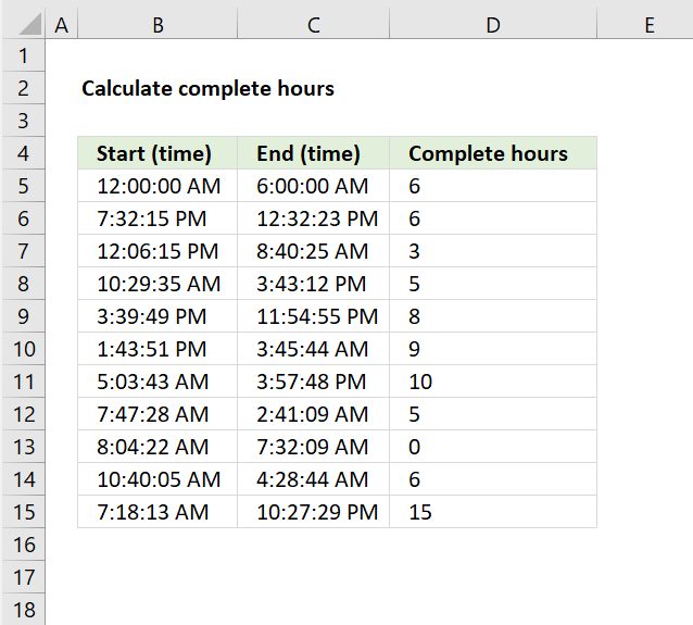
The formula in cell D5 calculates the number of complete hours between the time entries in cell B5 and C5.
Formula in cell D5:
Note that this formula works only with time entries, not date and time entries. It doesn't matter if the start time is past the end time, the formula will regardless return a positive hour value.
Explaining formula in cell D5
Step 1 - Subtract time entries
C5-B5
becomes
6:00:00 AM - 12:00:00 AM
Time entries in excel are actually a decimal value between 0 (zero) and 1. One hour is 1/24, six hours is 6/24 and so on.
0.25 - 0 equals 0.25
Step 2 - Remove sign
The ABS function removes the minus sign if it exists, the HOUR function can't calculate negative values.
ABS(C5-B5)
becomes
ABS(0.25) and returns 0.25.
Step 3 - Convert decimal to hour(s)
The HOUR function calculates hours based on a decimal value.
HOUR(ABS(C5-B5))
becomes
HOUR(0.25)
and returns 6.
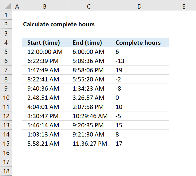
The image above demonstrates a formula the returns negative hours if the start time is later than the end time.
Formula in cell D5:
Explaining formula in cell D5
This part of the formula HOUR(ABS(C5-B5)) is explained above.
Step 1 - Calculate if end date is smaller than the start date
C5<B5
becomes
0.25<0
and returns FALSE.
Step 2 - Return -1 if TRUE and 1 if FALSE
IF(C5<B5,-1,1)
becomes
IF(0.25<0,-1,1)
becomes
IF(FALSE,-1,1) and returns 1.
Step 3 - Multiply with result
HOUR(ABS(C5-B5))*IF(C5<B5,-1,1)
becomes
6*IF(C5<B5,-1,1)
becomes
6*1 and returns 6 in cell D5.
8. Count complete hours between two date and time values
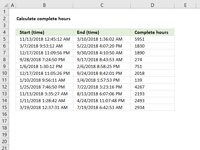
The picture above shows a formula that calculates complete hours between date and time entries.
Formula in cell D5:
If you want negative hours then remove the ABS function:
The TEXT function formats the result of C5-B5 into complete hours.
9. How to use the MINUTE function

What is the MINUTE function?
The MINUTE function returns a whole number that represents the minute based on an Excel time value. The returned number is an integer between 0 (zero) and 59.
What is an integer?
An integer is a whole number that can be positive, negative, or zero, but not a fraction or decimal. Excel can't calculate the minute based on negative integers.
What is an Excel time value?
Excel time is actually a decimal number ranging between 0 and 1 in Excel and then formatted as time.
For example, 12:00 PM is represented as 0.5 because it is half of a day, you can verify this by typing 12:00 PM in a cell and then change the cell formatting to general. This will show the value as Excel interprets it.
How does Excel recognize time values?
Excel recognizes certain text strings like "6:45 PM" as valid time values. A recognized time value is right aligned in the cell just like a regular number, shown in the image below in cell B2.
A time number that is not recognized is left aligned which is demonstrated in cell B4 in the image above. This visual feedback lets you easily spot values that need closer inspection.
What is a minute in an Excel time value?
There are 60 minutes in one hour and 24 hours in one day. 60 * 24 = 1440 minutes in one day.
1/1440 or approx. 0.000694 represents one minute in Excel time value. Excel uses a number 0 <= x <= 1 in decimal form to represent time in an Excel worksheet. 0 is zero minutes and 1 is 1440 minutes (24 hours).
Why is 1 day equal to 1440 minutes?
This has to do how Excel handles dates. Each date is represented by an integer and one day is equal to 1 in Excel. There are 24 hours or 1440 minutes in one day.
Dates are stored numerically but formatted to display in human-readable date/time formats, this enables Excel to do work with dates in calculations.
For example, dates are stored as sequential serial numbers with 1 being January 1, 1900 by default. The integer part (whole number) represents the date the decimal part represents the time.
This allows dates to easily be formatted to display in many date/time formats like mm/dd/yyyy, dd/mm/yyyy and so on and still be part of calculations as long as the date is stored numerically in a cell.
You can try this yourself, type 10000 in a cell, press CTRL + 1 and change the cell's formatting to date, press with left mouse button on OK. The cell now shows 5/18/1927.
Related functions
| Excel Function | Description |
|---|---|
| HOUR(time) | Returns the hour portion of a time value |
| MINUTE(time) | Returns the minute portion of a time value |
| SECOND(time) | Returns the second portion of a time value |
| TIME(hour,minute,second) | Creates a time value from hour, minute, and second values |
| TIMEVALUE(time_text) | Converts a text time to a serial time value |
MINUTE function Syntax
MINUTE(serial_number)
MINUTE function Arguments
| serial_number | Required. An Excel time value that you want to extract the minute from. |
MINUTE function example
This example demonstrates the MINUTE function in cell C3, it extracts the minute from the Excel time value specified in cell B3: "1:34:22 PM"
Formula in cell C3:
The MINUTE function returns 34.
MINUTE function not working

The MINUTE function returns #NUM! error if the decimal is a negative value.
The MINUTE function returns #VALUE! error if the Excel time value is invalid.
10. How to use the MONTH function

What is the MONTH function?
The MONTH function extracts the month as a number from an Excel date.
- 1 - January
- 2 - February
- 3 - March
- 4 - April
- 5 - May
- 6 - June
- 7 - July
- 8 - August
- 9 - September
- 10 - October
- 11 - November
- 12 - December
Table of Contents
1. MONTH Function Syntax
MONTH(serial_number)
2. MONTH Function Arguments
| serial_number | Required. The date value you want to extract the month from. |
3. MONTH Function not working

Check your spelling, the image above shows the MONTH function misspelled. An #NAME? error is shown in cell C3.

Cell B3 contains a text value and not a proper Excel date, this returns a #VALUE! error in cell C3.
4. MONTH Function example
Formula in cell C3:
To understand the MONTH function I need to explain that it needs an Excel date in order to calculate the month properly. The date in cell B3 is an Excel date meaning it is a number formatted as a date. 1 is 1/1/1900 and 1/1/2000 is 36526 meaning there are 36526 days between the dates.
You can verify this, select a cell containing 1/1/2000 and press CTRL + 1 to open the "Format Cells" dialog box.
The "Sample" shown in the image above demonstrates what the value changes to if you choose to format the cells using the category "General". The sample contains 36526 which is the number representing 1/1/2000.
5. MONTH Function alternative

Formula in cell C3:
Explaining formula
Step 1 - TEXT function
The TEXT function lets you format values.
TEXT(value, format_text)
value - The string you want to format. You can use a cell reference here or use a text string.
format_text - Formatting code allowing you to change the way, for example, a date or a number is displayed to the Excel user.
Step 2 - Populate arguments
The TEXT function has two arguments.
value - B3
format_text - "m"
"m" is an abbreviation for month. A single "m" returns the number representing the position of a given month in a year.
Check out this article to learn more about formatting codes in the TEXT function.
Step 3 - Evaluate TEXT function
TEXT(B3, "m")
becomes
TEXT(45089, "m")
and returns 6. 6 represents the sixth month in a year which is "June".
6. MONTH function - return month name instead of a number
6.1 Example 1 - INDEX function

Formula in cell C3:
Explaining formula in cell C3
Step 1 - Calculate month number
MONTH(B3)
- 1 - January
- 2 - February
- 3 - March
- 4 - April
- 5 - May
- 6 - June
- 7 - July
- 8 - August
- 9 - September
- 10 - October
- 11 - November
- 12 - December
MONTH(B3)
becomes
MONTH(45089)
and returns 6. Number 6 represents "June".
Step 2 - Return corresponding month name
The INDEX function returns a value in a cell range or array based on a row and column number (optional).
INDEX(array, [row_num], [column_num], [area_num])
INDEX({"January"; "February"; "March"; "April"; "May"; "June"; "July"; "August"; "September"; "October"; "November"; "December"},MONTH(B3))
becomes
INDEX({"January"; "February"; "March"; "April"; "May"; "June"; "July"; "August"; "September"; "October"; "November"; "December"}, 6)
and returns "June". "June" is the sixth month in a year.
6.2 Example 2 - TEXT function

Formula in cell C4:
Explaining formula in cell C4
The TEXT function lets you format values.
TEXT(value, format_text)
value - The string you want to format. You can use a cell reference here or use a text string.
format_text - Formatting code allowing you to change the way, for example, a date or a number is displayed to the Excel user.
Formatting code "mmmm" evaluates to the month name.
TEXT(B4, "mmmm")
becomes
TEXT(44603, "mmmm")
and returns "March".
6.3 Example 3 - Cell formatting

You can also show the month name using cell formatting, the image above demonstrates cell formatting applied to cell C5.
How to apply cell formatting:
- Select cell C5.
- Press CTRL + 1 to open the "Format Cells" dialog box.
- Press with left mouse button on "Category" Custom, see the image above.
- Enter mmmm below Type:
- Press with left mouse button on OK button to apply cahnges.
7. Filter dates based on month

Formula in cell D3:
Explaining formula
Step 1 - Calculate month number for each date value
MONTH(B3:B11)
becomes
MONTH({44667; 44667; 44700; 44707; 45006; 45051; 45054; 45075; 45079})
and returns {4; 4; 5; 5; 3; 5; 5; 5; 6}.
Step 2 - Compare month number to condition
The equal sign lets you check if values are equal, note that this does not perform a case-sensitive comparison. Check out the EXACT function if upper and lower letters matter.
MONTH(B3:B11)=5
becomes
{4; 4; 5; 5; 3; 5; 5; 5; 6}=5
and returns
{FALSE; FALSE; TRUE; TRUE; FALSE; TRUE; TRUE; TRUE; FALSE}
Step 3 - Extract dates meeting the condition
The FILTER function is a new function available to Excel 365 subscribers. It lets you extract values based on a condition or criteria.
FILTER(array, include, [if_empty])
FILTER(B3:B11, MONTH(B3:B11)=5)
becomes
FILTER({44667; 44667; 44700; 44707; 45006; 45051; 45054; 45075; 45079}, {FALSE; FALSE; TRUE; TRUE; FALSE; TRUE; TRUE; TRUE; FALSE})
and returns {44700; 44707; 45051; 45054; 45075}.
Compatibility Functions 13 Mar 2024 10:36 PM (2 years ago)

Table of Contents
- How to use the BETADIST function
- How to use the BETAINV function
- How to use the BINOMDIST function
- How to use the CHIDIST function
- How to use the CHIINV function
- How to use the CHITEST function
- How to use the CONFIDENCE functionartif
- How to use the COVAR function
- How to use the CRITBINOM function
- How to use the EXPONDIST function
- How to use the FDIST function
- How to use the FLOOR function
- How to use the FORECAST function
- How to use the FTEST function
- How to use the GAMMADIST function
- How to use the LOGNORMDIST function
- How to use the MODE function
- How to use the PERCENTRANK function
- How to use the QUARTILE function
- How to use the RANK function
- How to use the STDEV function
1. How to use the BETADIST function
What is the BETADIST function?
The BETADIST function calculates the cumulative beta distribution function representing an outcome in the form of probability.
What is the beta distribution?
The beta distribution is a continuous probability distribution defined over the interval [0, 1] and parameterized by two positive shape parameters, alpha (α) and beta (β).
What is a continuous probability distribution?
A continuous probability distribution is a function defined over a range of continuous values that provides the probability of a random variable falling between any two points, having a density described by an equation rather than discrete probabilities.
1.1 Syntax
BETADIST(x,alpha,beta,[A],[B])
1.2 Arguments
| x | Required. |
| alpha | Required. A parameter which determines the shape of the distribution. |
| beta | Required. A parameter which determines the shape of the distribution. |
| [A] | Optional. Lower bound, default value 0 (zero). |
| [B] | Optional. Upper bound, default value 1. |
What is a cumulative beta probability distribution?
The cumulative beta distribution function gives the probability that a beta-distributed random variable with parameters α and β will be less than or equal to a given value x, providing the accumulated area under the probability density curve from 0 to x.
When to use the beta distribution?
The beta distribution is used to model random variables limited to intervals of 0 to 1, such as binomial success probabilities, percentage or fraction outcomes, and measurements constrained between limits, making it useful in Bayesian statistics, experimental design, quality control studies, process monitoring, and other applications involving binary or fraction outcomes.
What are continuous values?
Continuous values are numbers that can take on any quantity within a range and can have infinitely many possibilities, unlike discrete values which have distinct separated values; continuous values can use intervals and ranges to describe events rather than fixed outcomes.
What are discrete probabilities?
Discrete probabilities are individual separated probabilities assigned to each of a countable number of possible outcomes that sum to 1, like rolling a die where each number has its own exact probability, as opposed to continuous distributions.
What are binomial success probabilities?
Binomial success probabilities describe the chance of a certain number of “successes” occurring in a fixed number of independent binary trial events modeled by the binomial distribution, like the probability of getting 3 heads in 10 coin flips.
What is Bayesian statistics?
Bayesian statistics is an approach to statistics using Bayes' theorem where prior beliefs about probabilities are updated as new evidence is acquired to determine conditional probabilities and update understanding of likelihood.
1.3 Example 1

The BETADIST function calculates the cumulative beta distribution representing an outcome in the form of probability between 0 and 1. The beta distribution is often used to model the uncertainty about the value of a probability or proportion when there is some prior information available.
Alpha is the number of successes plus one and beta is the number of failures plus one. Successes and failures is a generalization, it can be satisfied customers vs not satisfied customers or what ever you want.
A company manufactures a new product. The first 10 products has 7 working and 3 faulty. Assuming that the proportion of working products follows a beta distribution with parameters α = 8 and β = 4, what is the probability that more than 90% are working for the next products in line?
Alpha is the number of working products plus one and beta is the number of faulty products plus one. The ratio between the number of working products and the total number of products is 7/10 equals 0.7 The blue line has it's highest point at 0.7 if you check the x-axis.
The image above has argument
- x in cell C18 and that value is 0.9
- alpha in cell C19
- beta in cell C20
Formula in cell C24:
The formula in cell C24 returns approx. 0.981 which is the cumulative beta distribution meaning the area below the blue density probability function in the chart above up to x value 0.9
The value we are looking for is the area to the right of 0.9 which we can calculate by subtracting 0.947 with 1. 1 - 0.947 equals approx. 0.0185 or 1.85%
The probability that more than 90% are working is 1.85% The orange line in the chart displayed in the image above shows the cumulative value. As time goes by and more and more products are manufactured you can update the parameters of the beta distribution model to get a better probability value.
1.4 Example 2

This example continues on example 1 above. The company has now manufactured 100 products, 90 working and 10 defect.
The BETADIST function returns approx 0.570 which gives us 1 - 0.570 equals 0.430 or 43 %. This number 43% is the probability that the products to be manufactured in the future have 90% working and 10% defect.
This example shows that as the number of observations increases the probability density curve (blue) gets more narrow meaning the uncertainty is also decreasing. In other words, the function gets better at predicting the probability as the number of observations increases.
1.5 Example 3
The optional arguments [A] and [B] are lower and upper limits. The BETADIST function uses these limits to calculate the percentage value, a number between 0 and 1.
You will get the same result if you calculate the percentage yourself, here is an example.
The arguments are:
- x = 30
- alpha = 90
- beta = 110
- [A] = 15
- [B] = 45
Formula in cell C7:
The formula in cell C7 returns 0.922 which is 92.2 %. To calculate the percentage (x) we calculate the ratio between x and the total of the upper and lower limit.
30/(15+45) equals 30/60 = 0.5 We can use this number in the BETADIST function without the upper and lower limit and check if we get the same result.
=BETADIST(0.5,90,110)
returns 0.921957262116145 which is the exact same value as above (0.921957262116145).
1.6 Function not working
The BETADIST function returns
- #VALUE! error value if any argument is non-numeric.
- #NUM! error value if:
- alpha <= 0
- beta <= 0
- x < A
- x >B
- A = B
1.7 How is the function calculated?
The general equation to calculate the beta distribution:
2. How to use the BETAINV function
What is the BETAINV function?
The BETAINV function calculates the inverse of a cumulative beta distribution. The beta distribution can help estimate how long a project might take by using the expected finish time and how variable the timeline could be. It gives the chance the project will be done at different dates based on the variability.
This function is outdated and replaced by the BETA.INV function which was introduced in Excel 2010.
The BETAINV function may not be available in future Excel versions and Microsoft recommends using the newer function from now on.
What is the inverse of the cumulative beta distribution?
The inverse of the cumulative beta distribution is a function that returns the value of x for a given probability p and parameters α and β of the beta distribution.
What is a cumulative beta probability distribution?
The cumulative beta distribution function gives the probability that a beta-distributed random variable with parameters α and β will be less than or equal to a given value x, providing the accumulated area under the probability density curve from 0 to x.
What is a beta probability density distribution?
A beta probability density distribution is a function whose shape over [0,1] depends on parameters α and β that gives the relative likelihood of a beta-distributed random variable occurring at different points, whose total area under the curve integrates to 1.
What are continuous values?
Continuous values are numbers that can take on any quantity within a range and can have infinitely many possibilities, unlike discrete values which have distinct separated values; continuous values can use intervals and ranges to describe events rather than fixed outcomes.
What are discrete probabilities?
Discrete probabilities are individual separated probabilities assigned to each of a countable number of possible outcomes that sum to 1, like rolling a die where each number has its own exact probability, as opposed to continuous distributions.
What are binomial success probabilities?
Binomial success probabilities describe the chance of a certain number of “successes” occurring in a fixed number of independent binary trial events modeled by the binomial distribution, like the probability of getting 3 heads in 10 coin flips.
What is Bayesian statistics?
Bayesian statistics is an approach to statistics using Bayes' theorem where prior beliefs about probabilities are updated as new evidence is acquired to determine conditional probabilities and update understanding of likelihood.
2.1 Syntax
BETAINV(probability,alpha,beta,[A],[B])
2.2 Arguments
| probability | Required. |
| alpha | Required. A parameter which determines the shape of the distribution. |
| beta | Required. A parameter which determines the shape of the distribution. |
| [A] | Optional. Lower bound, default value 0 (zero). |
| [B] | Optional. Upper bound, default value 1. |
What is alpha and beta in a beta distribution?
The beta distribution is very flexible due to how alpha and beta shape its variance and skew. Changing their values gives a wide range of distribution shapes. In the beta distribution, alpha and beta are shape parameters that control the form of the distribution:
Alpha (α): Controls the height of the peak. Higher alpha = taller, more concentrated peak. Alpha mainly changes the peak height.
Beta (β): Controls the tails of the distribution. Higher beta = shorter, thinner tails. Beta mainly changes the tail thickness.
As α & β > 1, shape becomes more symmetric and bell-shaped.
As α & β < 1, shape becomes asymmetrical and J or U shaped.
When α = β = 1, the distribution becomes uniform.
They allow modeling different levels of variance and asymmetry.
2.3 Example 1

The BETAINV function calculates the inverse of the cumulative beta distribution representing an outcome in the form of probability between 0 and 1.
The BETADIST function is related to the BETAINV function: BETAINV(probability,alpha,beta,[A],[B]) = x
BETADIST(x,alpha,beta,[A],[B]) = probability
A company manufactures a new product. The first 10 products has 7 working and 3 faulty. Assuming that the proportion of working products follows a beta distribution with parameters α = 8 and β = 4, find the values of the proportion corresponding to the 2.5th and 97.5th percentiles?
Alpha is the number of working products plus one and beta is the number of faulty products plus one. The ratio between the number of working products and the total number of products is 7/10 equals 0.7 The blue line has it's highest point at 0.7 if you check the x-axis.
The image above has argument
- probability in cell C18 and that value is 0.975
- alpha in cell C19
- beta in cell C20
Formula in cell C10:
The formula returns approx. 0.891 for a probability of 97.5% and approx. 0.390 for a probability of 2.5%.
2.4 Example 2

This example continues on example 1 above. The company has now manufactured 100 products, 90 working and 10 defect.
Assuming that the proportion of working products follows a beta distribution with parameters α = 91 and β = 11, find the values of the proportion corresponding to the 2.5th and 97.5th percentiles?
The BETAINV function returns 0.944 for 97.5% and 0.825 for 2.5 %.
This example shows that as the number of observations increases the probability density curve (blue) gets more narrow meaning the uncertainty is also decreasing. In other words, the function gets better as the number of observations increases.
2.5 Example 3

The optional arguments [A] and [B] are lower and upper limits respectively. The BETAINV function uses these limits to assist you calculating the x value for you which is a number between the lower limit and the upper limit.
You will get the same result if you calculate the x value yourself, here is an example.
The arguments are:
- probability = 0.921957262116145
- alpha = 90
- beta = 110
- [A] = 15
- [B] = 45
Formula in cell C7:
The formula in cell C7 returns 30.You can calculate x using only three arguments probability, alpha, and beta. Multiply the result with the total of the upper and lower limit to calculate x. It will be somewhere between the limits. Here is how:
=BETAINV(0.921957262116145,90,110)
returns 0.5
0.5*(15+45)=30 which is exactly what the function returns in cell C24
2.6 Function not working
The BETAINV function returns a:
- #VALUE! error value if any argument is non-numeric.
- #NUM! error value if:
- alpha <= 0 (zero)
- beta <= 0 (zero)
- probability <= 0 (zero)
- probability > 1
- A = B
3. How to use the BINOMDIST function

What is the BINOMDIST function?
The BINOMDIST function calculates the individual term binomial distribution probability, use this function when
- the success probability is constant through all trials
- you know the number of trials
- the outcome is either a success or failure
- each trial is independent of the other trials.
What is the binomial distribution probability?
The binomial distribution probability gives the likelihood of a specific number of successes occurring in a fixed number of independent trials, each having the same binary success/failure probability.
What is the individual term binomial distribution probability?
The individual term binomial distribution probability is the probability of exactly k successes in n trials with a given success probability p, calculated using combinations to determine the number of ways k successes can occur in those trials.
What are combinations?
A combination is a way of selecting items from a collection where the order of selection does not matter.
For example, if you have three fruits, say an apple, an orange, and a pear. There are three combinations of two that can be drawn from this set:
- apple and a pear
- apple and an orange
- pear and an orange
3.1 Syntax
BINOMDIST(number_s,trials,probability_s,cumulative)
3.2 Arguments
| number_s | Required. The number of successful tests. |
| trials | Required. How many independent tests. |
| probability_s | Required. The probability of success in each test. |
| cumulative | Required. A boolean value. TRUE - cumulative distribution function FALSE - probability mass function |
What is cumulative binomial distribution?
The cumulative binomial distribution function gives the probability that a binomial random variable with a given number of trials and success probability will take on a value less than or equal to a specified number of successes x.
What is probability mass function?
A probability mass function is a function that defines a discrete probability distribution by providing the probability that each of a countable number of possible discrete outcomes will occur for a random variable.
What is a binomial random variable?
A binomial random variable is a discrete random variable that represents the number of "successes" in a fixed number of independent binary trials, where each trial has the same probability of success.
What are discrete probabilities?
Discrete probabilities are individual separated probabilities assigned to each of a countable number of possible outcomes that sum to 1, like rolling a die where each number has its own exact probability, as opposed to continuous distributions.
3.3 Example 1
The probability that a customer accepts an offer is estimated to be 60%. The offer is given to 20 customers. What is the probability that at most 12 of them accepts the offer?
To solve this we need to use the binomial distribution. It models the number of successes in a fixed number of independent trials (20 customers). Each trial has the same probability of success (0.6 or 60%).
Let x be the random variable representing the number of customers who accepts the offer. Then x follows a binomial distribution with parameters n = 20 (number of trials) and p = 0.6 (probability of success).
The probability we want to find is P(x ≤ 12) which is the cumulative probability of the binomial distribution from 0 up to 12.
Formula in cell C8:
The formula returns approx. 0.5841, in other words, the probability is 58.4% that up to 12 customers accepts the offer.
The chart in the image above shows an orange line representing the cumulative probability. Go to 12 on the x-axis and find where the orange line intersects the middle of the column. The secondary y-axis to the right shows a value just below 0.6 which seems to match the calculated number 0.5841
3.4 Example 2

There are 22 machines that operate independently of each other in a factory. The probability of a breakdown occurring during a day is 0.1 for each of the machines. What is the probability that three machines will stop during a certain day?
The binomial distribution is what we need in this example. It models the number of successes (machine breakdowns) in a fixed number of independent trials (22 machines), where each trial has the same probability of success (0.1 or 10%).
Let x be the random variable representing the number of machines that break down during the day. Then x follows a binomial distribution with parameters n = 22 (number of machines) and p = 0.1 (probability of breakdown for each machine).
The probability we want to find is P(X = 3), which is the probability mass function of the binomial distribution evaluated at 3.
The formula returns 0.208, in other words, the probability is 20.8% that exactly 3 machines break down during a day.
The chart in the image above shows blue chart columns representing the probability mass function of the binomial distribution. Go to 3 on the x-axis and find the value value for that column. The y-axis to the left shows a value just above 0.2 which seems to match the calculated number 0.208
3.5 Example 3

There are 30 students in a class. There is a 50% risk that each student, independently of each other, will catch a harmless but highly contagious cold. What is the chance that 12 students or less will attend school on the same day?
We need to find the probability that 12 or fewer students will not catch the cold, which is the same as the probability that 18 or more students will catch the cold.
- Total number of students: 30
- Probability of catching the cold for each student: 0.5 (or 50%)
We want to find P(X ≥ 18), which is the probability that 18 or more students will catch the cold.
P(X ≥ 18) = 1 - P(X ≤ 17)
We can calculate P(X ≤ 17) using the cumulative distribution function of the binomial distribution and then take the complement to find P(X ≥ 18).
Formula in cell C21:
The formula in cell C21 returns 0.181 which is 18.1%. This means that there is a 18.1% chance that 12 students or less will attend school on the same day.
3.6 Function not working
The BINOMDIST function returns
- #VALUE! error value if number_s, trials or probability_s argument is non-numeric.
- #NUM! error value if:
- number_s <= 0 (zero)
- number_s > trials
- probability_s < 0 (zero)
- probability_s > 1
- A = B
number_s and trials are converted into integers.
4. How to use the CHIDIST function
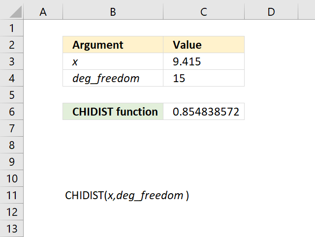
The CHIDIST function calculates the right-tailed probability of the chi-squared distribution. Use this function to check if a hypothesize is valid.
What is a chi-squared distribution?
The chi-squared distribution is a theoretical probability distribution modeling the sum of squared standard normal random variables used in inferential statistics for estimation, confidence intervals, and hypothesis testing.
What is the probability of the chi-squared distribution?
The probability of the chi-squared distribution determines the likelihood that the sum of squared standard normal variables will take on a value less than or equal to a given number, depending on its degrees of freedom parameter.
What is a hypothesize?
In statistics, a hypothesis is an assumption about some aspect of a population parameter or probability model that can be tested using observations and data to determine if there is sufficient evidence in the sample to support the assumed hypothesis.
What is a cumulative chi-squared distribution?
The cumulative chi-squared distribution function gives the probability that the sum of squared standard normals will result in a value less than or equal to a specified number x, giving the accumulated area under the probability density curve.
What is a probability density function of a chi-squared distribution?
A chi-squared probability density function is a function that defines the relative likelihood of different outcomes for the sum of squared standard normals based on its degrees of freedom parameter, integrating to a total area of 1 over the domain.
What is inferential statistics for estimation?
Inferential statistics for estimation involve using a random sample to estimate characteristics and parameters about a larger population using statistical techniques like confidence intervals and point estimation to quantify uncertainty about the estimates.
What is confidence intervals?
A confidence interval provides a range of plausible values for an unknown population parameter centered around a sample estimate, describing the uncertainty around the estimate at a specified level of confidence.
What is the sum of squared standard normal variables?
The sum of squared standard normal variables refers to summing multiple independent normally distributed random variables each with a mean of 0 and variance of 1, which results in a chi-squared distribution that can be used for statistical modeling and analysis.
4.1 Syntax
CHIDIST(x,deg_freedom)
4.2 Arguments
| x | Required. A numerical value representing a point in the probability distribution you want to be evaluated. |
| deg_freedom | Required. A numerical value representing the degrees of freedom. |
deg_freedom argument is converted into integers.
What are the degrees of freedom?
The degrees of freedom in a chi-squared distribution refers to the number of standard normal random variables being squared and summed, which affects the shape of the distribution and occurs in statistical tests as the sample size minus the number of estimated parameters.
What is a boolean value?
A Boolean value is a logical data type having only two possible states - true or false - which logic gates and circuits are based on.
4.3 Example 1

The CHIDIST function calculates the right-tailed probability of a given x value based on the chosen number of degrees of freedom. This means that the right-tailed probability represents the area below the orange line from a given x value to infinity.
For example, the image above shows a chart containing two lines colored blue and orange.
- Blue line - chi squared density probability function
- Orange line - cumulative chi-squared distribution
Both lines represents a chi-squared distribution with 1 degree of freedom. The formula in cell C20 contains the CHIDIST function, it calculates the probability based on the following arguments:
- x - 2
- deg_freedom - 1
Formula in cell C20:
=CHIDIST(C16,C17)
It returns 0.157299207050285 which represents the area below the orange line from x value = 2 and to infinity. You can also find that value if you find number 2 on the x-axis and then locates the value on the y-axis where x value 2 intersects the blue line which is somewhere around 0.85
0.85 is the left tailed cumulative probability for the chi squared distribution with 1 degree of freedom, however, the right-tailed probability is easy to calculate. We need to find the complement which we can calculate by subtracting 1 with 0.85 This results in 1 - 0.85 = 0.15 which is approx. 0.157299207050285
4.4 Example 2

What is the right-tailed probability for a chi-squared distribution with two degrees of freedom for an x value of 3?
The CHIDIST function has two arguments:
- x - which is specified in cell C16 and is 3 in this example.
- deg_freedom - The degree of freedom is 2 and is specified in cell C17.
The image above shows a chart demonstrating both the cumulative chi-squared distribution (blue line) and the density probability function (orange line) between x values of 0 to 10. These distribution lines change based on the degree of freedom value. In this example the two lines has 2 degrees of freedom.
Formula in cell C20:
The formula in cell C20 returns approx. 0.223. This value can be found in the chart above. First we need to calculate the complement to 0.223 which is 1- 0.223 = 0.777
The orange line shows the density probability function, the x value is found on the x-axis. 3 on the x-axis corresponds to the 0.777 value on the y-axis based on the intersection between the blue line and x value 3.
4.5. Example 3

What is the right-tailed probability for a chi-squared distribution with eight degrees of freedom for an x value of 6?
The CHIDIST function has two arguments:
- x - which is specified in cell C16 and is 6 in this example.
- deg_freedom - The degree of freedom is 8 and is specified in cell C17.
The image above shows a chart demonstrating both the cumulative chi-squared distribution (blue line) and the density probability function (orange line) between x values of 0 to 10. These distribution lines change based on the degree of freedom value. In this example the two lines has 8 degrees of freedom.
Formula in cell C20:
The formula in cell C20 returns approx. 0.65. This value can be found in the chart above. First we need to calculate the complement to 0.65 which is 1- 0.65 = 0.35
The orange line shows the density probability function, the x value is found on the x-axis. 6 on the x-axis corresponds to the 0.35 value on the y-axis based on the intersection between the blue line and x value 6.
4.6. Function not working
The CHIDIST function returns
- #VALUE! error value if x or deg_freedom argument is non-numeric.
- #NUM! error value if:
- x < 0 (zero)
- deg_freedom < 1
- deg_freedom > 10^10
5. How to use the CHIINV function

What is the CHIINV function?
The CHIINV function calculates the inverse of the right tailed probability of the chi-squared distribution.
What is a chi-squared distribution?
The chi-squared distribution is a theoretical probability distribution modeling the sum of squared standard normal random variables used in inferential statistics for estimation, confidence intervals, and hypothesis testing.
What is the probability of the chi-squared distribution?
The probability of the chi-squared distribution determines the likelihood that the sum of squared standard normal variables will take on a value less than or equal to a given number, depending on its degrees of freedom parameter.
What is a hypothesize?
In statistics, a hypothesis is an assumption about some aspect of a population parameter or probability model that can be tested using observations and data to determine if there is sufficient evidence in the sample to support the assumed hypothesis.
What is inferential statistics for estimation?
Inferential statistics for estimation involve using a random sample to estimate characteristics and parameters about a larger population using statistical techniques like confidence intervals and point estimation to quantify uncertainty about the estimates.
What is confidence intervals?
A confidence interval provides a range of plausible values for an unknown population parameter centered around a sample estimate, describing the uncertainty around the estimate at a specified level of confidence.
What is the left-tailed probability of the chi-squared distribution?
The left-tailed probability of the chi-squared distribution gives the chance that the sum of squared standard normals is less than or equal to a specified value x, focusing only on the lower portion of outcomes under the density curve.
What is the inverse of a left-tailed probability of the chi-squared distribution?
The inverse of a left-tailed chi-squared probability determines the value x that corresponds to a given cumulative probability for the lower tail, calculating the sum of squares threshold that captures the specified proportion of possible outcomes.
What is the difference between the CHIDIST and CHINV functions?
The CHIDIST and CHINV functions are related.
CHIDIST(x, deg_freedom) = probability
then
CHINV(probability , deg_freedom) = x
5.1 Syntax
CHIINV(probability,deg_freedom)
5.2 Arguments
| probability | Required. A numerical value representing the probability with the chi-squared distribution. |
| deg_freedom | Required. A numerical value representing the degrees of freedom. |
What are the degrees of freedom?
The degrees of freedom in a chi-squared distribution refers to the number of standard normal random variables being squared and summed, which affects the shape of the distribution and occurs in statistical tests as the sample size minus the number of estimated parameters.
5.3 Example 1
What is x for the right-tailed probability of 0.317310507862914 with 1 degree of freedom?
The image above shows a chart displaying the chi square distribution for a degree of freedom of 1. The blue line is the cumulative chi square distribution and the orange line is the density probability function.
Below the chart are the arguments specified:
- probability : 0.317310507862914
- deg_freedom : 1
The formula in cell C20 calculates the inverse (x) of the right-tailed probability of the chi-squared distribution based on the specified arguments above. This means the area below the orange line from x value = 1 to infinity.
Formula in cell C20:
This means that 0.317310507862914 represents the area below the orange line from x value = 1 to infinity.
0.317310507862914 is the right-tailed probability value, to calculate the left-tailed probability we need the complement. We subtract 1 with 0.317310507862914 which equals 0.682689492137086
We can now find the probability value (0.6827) on the y-axis, then find where the cumulative chi square distribution which is the blue line intersects 0.6827. Now find the x value on the x-axis which is 1 based on the intersection of the blue line and y-axis value 0.6827. This value matches the calculated value in cell C20.
Cell C21 contains the CHIDIST function, it calculates the right-tailed probability based on the calculated value in cell C20, the number of degrees of freedom specified in cell C17 which corresponds to the cumulative chi square distribution.
The value in cell C21 matches the value in cell C16 which demonstrates the relation between the CHIDIST function and the CHIINV function.
5.4 Example 2

What is x for the right-tailed probability of 0.22313016014843 with 2 degrees of freedom?
The image above shows a chart displaying the chi square distribution for 2 degrees of freedom. The blue line is the cumulative chi square distribution and the orange line is the density probability function.
Below the chart are the arguments specified:
- probability : 0.22313016014843
- deg_freedom : 2
The formula in cell C20 calculates the inverse (x) of the right-tailed probability of the chi-squared distribution based on the specified arguments above.
Formula in cell C20:
This means that 0.22313016014843 represents the area below the orange line from x value = 3 to infinity.
0.22313016014843 is the right-tailed probability value, to calculate the left-tailed probability we need the complement. We subtract 1 with 0.22313016014843 which equals 0.77686983985157
We can now find the probability value (0.7769) on the y-axis, then find where the cumulative chi square distribution which is the blue line intersects 0.7769. Now find the x value on the x-axis which is 3 based on the intersection of the blue line and y-axis value 0.7769. This value matches the calculated value in cell C20.
Cell C21 contains the CHIDIST function, it calculates the right-tailed probability based on the calculated value in cell C20, the number of degrees of freedom specified in cell C17 which corresponds to the cumulative chi square distribution.
The value in cell C21 matches the value in cell C16 which demonstrates the relation between the CHIDIST function and the CHIINV function.
5.5 Example 3

What is x for the right-tailed probability of 0.433470120366709 with 8 degrees of freedom?
The image above shows a chart displaying the chi square distribution for 8 degrees of freedom. The blue line is the cumulative chi square distribution and the orange line is the density probability function.
Below the chart are the arguments specified:
- probability : 0.433470120366709
- deg_freedom : 8
The formula in cell C20 calculates the inverse (x) of the right-tailed probability of the chi-squared distribution based on the specified arguments above.
Formula in cell C20:
This means that 0.433470120366709 represents the area below the orange line from x value = 8 to infinity.
0.22313016014843 is the right-tailed probability value, to calculate the left-tailed probability we need the complement. We subtract 1 with 0.22313016014843 which equals 0.77686983985157
We can now find the probability value (0.7769) on the y-axis, then find where the cumulative chi square distribution which is the blue line intersects 0.7769. Now find the x value on the x-axis which is 8 based on the intersection of the blue line and y-axis value 0.7769. This value matches the calculated value in cell C20.
Cell C21 contains the CHIDIST function, it calculates the right-tailed probability based on the calculated value in cell C20, the number of degrees of freedom specified in cell C17 which corresponds to the cumulative chi square distribution.
The value in cell C21 matches the value in cell C16 which demonstrates the relation between the CHIDIST function and the CHIINV function.
5.6. Function not working
The CHIINV function returns
- #VALUE! error value if probability or deg_freedom argument is non-numeric.
- #NUM! error value if:
- probability < 0 (zero)
- probability > 1 (zero)
- deg_freedom < 1
deg_freedom argument is converted into integers if necessary.
6. How to use the CHITEST function
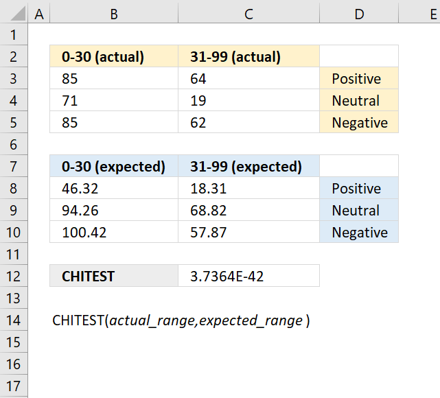
The CHITEST function calculates the test for independence, the value returned from the chi-squared statistical distribution and the correct degrees of freedom. Use this function to check if hypothesized results are valid.
What is a test for independence?
A test for independence is a statistical hypothesis test that checks if two categorical variables are related or independent based on observed data, commonly done using Pearson's chi-squared test or G-test to compare observed and expected frequency counts.
What is a chi-squared distribution?
The chi-squared distribution is a theoretical probability distribution modeling the sum of squared standard normal random variables used in inferential statistics for estimation, confidence intervals, and hypothesis testing.
What is the probability of the chi-squared distribution?
The probability of the chi-squared distribution determines the likelihood that the sum of squared standard normal variables will take on a value less than or equal to a given number, depending on its degrees of freedom parameter.
What is an hypothesis?
In statistics, a hypothesis is an assumption about some aspect of a population parameter or probability model that can be tested using observations and data to determine if there is sufficient evidence in the sample to support the assumed hypothesis.
What is a cumulative chi-squared distribution?
The cumulative chi-squared distribution function gives the probability that the sum of squared standard normals will result in a value less than or equal to a specified number x, giving the accumulated area under the probability density curve.
What is a probability density function of a chi-squared distribution?
A chi-squared probability density function is a function that defines the relative likelihood of different outcomes for the sum of squared standard normals based on its degrees of freedom parameter, integrating to a total area of 1 over the domain.
What is inferential statistics for estimation?
Inferential statistics for estimation involve using a random sample to estimate characteristics and parameters about a larger population using statistical techniques like confidence intervals and point estimation to quantify uncertainty about the estimates.
What is confidence intervals?
A confidence interval provides a range of plausible values for an unknown population parameter centered around a sample estimate, describing the uncertainty around the estimate at a specified level of confidence.
What is the sum of squared standard normal variables?
The sum of squared standard normal variables refers to summing multiple independent normally distributed random variables each with a mean of 0 and variance of 1, which results in a chi-squared distribution that can be used for statistical modeling and analysis.
What are the degrees of freedom?
The degrees of freedom in a chi-squared distribution refers to the number of standard normal random variables being squared and summed, which affects the shape of the distribution and occurs in statistical tests as the sample size minus the number of estimated parameters.
6.1. Syntax
CHITEST(actual_range,expected_range)
6.2. Arguments
| actual_range | Required. A range of data. |
| expected_range | Required. A range of data. |
6.3. Example
How to check if hypothesized results are valid when using the CHISQ.TEST function?
To check if results from the CHISQ.TEST function are valid, look at the calculated test statistic and compare it to the critical value from the chi-squared distribution with degrees of freedom equal to (number of rows - 1) * (number of columns - 1) at the desired significance level, rejecting independence if the test statistic exceeds the critical value.
Formula in cell C12:
6.4. Example 2

In an archaeological study, researchers have collected data on the frequencies of different types of artifacts found at various excavation sites. They want to test if the observed frequencies of artifact types differ significantly from the expected frequencies based on historical records or theoretical models.
Observed frequencies of artifact types:
| Artifact types | Frequency: |
| A | 432 |
| B | 312 |
| C | 613 |
| D | 171 |
The theoretical probabilities for the artifacts are as follows:
| Artifact types | Probabilities |
| A | 0.25 |
| B | 0.18 |
| C | 0.41 |
| D | 0.16 |
Evaluate if the observed frequencies of artifact types deviate significantly from the expected frequencies.
Formula in cell C23:
Formula in cell D27:
Copy cell D27 to cells below as far as needed.
Formula in cell C32:
The CHISQ.TEST function returns 1.848E-07
Formula in cell C33:
Formula in cell C34:
The χ2 statistic for the observed frequencies is approx. 34.14 with 3 degrees of freedom. This is higher than the decision rule calculated in cell C34. The observed frequencies does differ significantly from the expected frequencies.
6.5. Function not working
Independence is indicated by a low number of χ2.
The CHITEST function returns
- #N/A error value if the number of data points in the arguments doesn't match.
6.6. How is the CHITEST Function calculated?
CHITEST function equation:
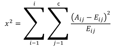
Aij = actual frequency in the i-th row, j-th column
Eij = expected frequency in the i-th row, j-th column
r = number of rows
c = number of columns
7. How to use the CONFIDENCE function

What is the CONFIDENCE function?
The CONFIDENCE function calculates the confidence interval for a population mean, using a normal distribution.
There are newer better functions that may have improved accuracy, this function is available for compatibility with older workbooks created in earlier Excel versions and other older software.
The new CONFIDENCE.NORM function and the CONFIDENCE.T function replace the older CONFIDENCE function which have better accuracy and improved functionality, Microsoft informs that the CONFIDENCE function may not be available in future Excel versions and recommends using the CONFIDENCE.NORM or the CONFIDENCE.T from now on.
What is a confidence interval?
A confidence interval is a range of values used to estimate a population parameter based on a sample statistic. It is constructed using a point estimate (such as the sample mean) plus or minus a margin of error.
The confidence level indicates the probability that the true population parameter lies within the interval. 90%, 95% and 99% confidence levels are commonly used. Useful for quantifying the uncertainty and potential error in statistics, surveys, polls, etc.
What is a population sample?
A population sample in statistics refers to a subset of data points selected from a larger population. The sample is a portion drawn from the total population.
It is studied to make inferences about the whole population, a sample aims to represent the population characteristics. The sample should be chosen randomly when possible to avoid bias.
The sample size should be adequate to represent the population, larger samples produce more precise results. Sampling reduces the cost and effort of studying the entire population and results are subject to sampling error due to studying a subset only.
How to pick a sample size to represent the population?
A typical starting point is to sample 5-10% of a large population or 20-30% of a small population. Statistical equations using confidence level, margin of error, and variance can precisely calculate the optimal sample size.
The goal is to pick a sample size large enough to produce a reasonable margin of error and desired power at a given confidence level. Higher confidence in the results requires a larger sample. Common levels are 90%, 95%, 99%.
The amount of potential error tolerated in results. Lower margin needs a larger sample. Larger populations require a bigger sample. Smaller populations need a higher sampling percentage. Bigger samples require more time, money and effort. Need to balance accuracy and feasibility.
What is a population mean?
The population mean is the average value of a quantitative variable calculated across an entire population also called the expected value or population average.
It is calculated by summing all the values in the population and dividing by the total number of individuals and is represented by the Greek letter μ (mu).
What is a normal distribution?

The normal distribution is a symmetric bell-shaped probability distribution described by its mean and standard deviation. Used by many to model a plethora of natural phenomena and represent unknown processes.
7.1. Syntax
CONFIDENCE(alpha, standard_dev, size)
7.2. Arguments
| alpha | Required. The significance level used to calculate the confidence level. 0.05 represents a 95% confidence level. |
| standard_dev | Required. The standard deviation for the data points. |
| size | Required. The number of data points. |
7.3. Example 1
A quality control manager at a manufacturing plant wants to determine the acceptable range of tensile strengths for a particular type of steel cable. They have recorded the tensile strengths of 25 randomly selected steel cable samples. Calculate the 90% confidence interval for the mean tensile strength of the steel cables.
The CONFIDENCE function lets you calculate the interval that satisfies a given a significance level, standard deviation and a number representing the population size.
The image above shows the argument:
- alpha in cell C19 which is 1-0.90 = 0.1
- standard_dev in cell C20 = 9.5
- size in cell C21 = 25
- Mean μ = 80
Formula in cell B6:
The CONFIDENCE function returns 3.1252218912078 for the specified arguments above.We can now calculate the upper and lower limit by adding the confidence interval from cell C23 to the mean μ. I have done this in cell C25:
The lower limit is calculated by subtracting the confidence level to the mean μ. Cell 26:
There is a 90% probability that the mean μ is between approx. 76.87 and approx. 83.13
7.4. Example 2

A researcher wants to estimate the average height of male students in a university. They take a random sample of 30 male students and measure their heights. Using the sample data, calculate the 95% confidence interval for the mean height of male students in the university.
Formula in cell B6:
The CONFIDENCE function lets you calculate the interval that satisfies a given a significance level, standard deviation and a number representing the population size.
The image above shows the argument:
- alpha in cell C19 which is 1-0.95 = 0.05
- standard_dev in cell C20 = 12
- size in cell C21 = 30
- Mean μ = 175
Formula in cell B6:
The CONFIDENCE function returns 4.29 for the specified arguments above.We can now calculate the upper and lower limit by adding the confidence interval from cell C23 to the mean μ. I have done this in cell C25:
The lower limit is calculated by subtracting the confidence level to the mean μ. Cell 26:
There is a 95% probability that the mean μ is between approx. 170.71 and approx. 179.29
7.5. Function not working
The CONFIDENCE function returns an
- #VALUE! error if an argument is not a number.
- #NUM! if alpha is less than 0 (zero) or more than 1.
8. How to use the COVAR function
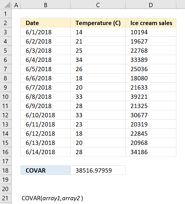
What is the COVAR function?
The COVAR function calculates the covariance meaning the average of the products of deviations for each pair in two different datasets.
What is covariance?
Covariance describes if two variables are connected meaning they rise together or if one decreases as the other increases. In other words, covariance measures how two random variables or datasets vary together.
Covariance is the average of the products of deviations for each pair in two different datasets. The covariance is positive if greater values in the first data set correspond to greater values in the second data set. The covariance is negative if greater values in the first data set correspond to smaller values in the second data set.
What is the average of the products of deviations for each pair in two different datasets?
The covariance between two datasets is computed by taking each data point, finding its deviation from its respective dataset mean by subtracting the mean, multiplying the two datasets' deviations together for each pair, and averaging these cross-products of deviations.
What is deviation?
In statistics, deviation is a measure of how far each value in a data set lies from the mean (the average of all values). A high deviation means that the values are spread out widely, while a low deviation means that they are clustered closely around the mean.
What is the mean?
It is also known as the average. It is calculated by adding up all the values in the data set and dividing by the number of values.
For example, if you have a data set of 5, 7, 9, 11, and 13, the mean is (5 + 7 + 9 + 11 + 13) / 5 = 9.
How to interpret covariance?

A positive covariance means that the variables tend to increase or decrease together indicating a positive linear relationship. The top left chart above shows variables with a positive covariance.
A negative covariance means that the variables tend to move in opposite directions indicating a negative linear relationship. The bottom left chart above shows variables with a negative covariance.
A zero covariance means that the variables are independent and have no linear relationship. The top and bottom right charts shows data with no linear relationship, the covariance is close to zero.
However, covariance is not a standardized measure and it depends on the scale and units of the variables. It is not easy to compare the covariances of different pairs of variables or interpret the strength of the relationship. A more common and useful measure of linear relationship is the correlation coefficient, which is the normalized version of covariance.
How to calculate normalized version of covariance?
To calculate the normalized version of covariance, which is also known as the correlation coefficient, you need to divide the covariance by the product of the standard deviations of the two variables. The standard deviation is a measure of how much the values in a data set deviate from the mean.

The correlation coefficient tells you also how much related the pairs are, this is not the case with the measure of covariance. The image above shows two charts, the data set in the right chart is identical to the left chart except they are ten times larger. Covariance is much larger for the right chart.
See the CORREL function for more.
8.1. Syntax
COVAR(array1, array2)
8.2. Arguments
| array1 | Required. The first data set. |
| array2 | Required. The second data set. |
8.3. Example
Formula in cell C18:
8.4. Function not working
Text, logical or empty values are ignored, however, 0 (zeros) are included.
The COVAR function returns
- #N/A error value if the number of data points in array1 and array2 is not equal.
- #DIV/0! error value if either array1 or array2 is empty.
8.5 How is the COVARIANCE.P Function calculated

To calculate the covariance for a population follow these steps:
- Calculate the mean of group of numbers named:
x="Temp"
y="Icecream"
For example:
Mean of X = x̄ is calculated in cell C10
Mean of Y = ȳ is calculated in cell D10 - For each data point xi and yi calculate the deviations from the mean.
Deviation of xi = xi - x̄ are calculated in cells E3:E9
Deviation of yi = yi - ȳ are calculated in cells F3:F9 - Multiply the deviations between each data point pair to get their products.
For each pair: (xi - x̄) * (yi - ȳ) are calculated in cells G3:G9 - Sum all the deviation products.
S = Σ(xi - x̄)(yi - ȳ) calculated in cell G10 - The covariance is the sum of products divided by the number of samples.
The equation for COVARIANCE.P is:

COVARIANCE.P(x,y) = (Σ(xi - x̄)(yi - ȳ))/n
x̄ is the sample means AVERAGE(array1)
ȳ is the sample means AVERAGE(array2)
n is the sample size.
9. How to use the CRITBINOM function

How to use the CRITBINOM function?
The CRITBINOM function calculates the minimum value for which the binomial distribution is equal to or greater than a given threshold value.
The CRITBINOM function is outdated and has been replaced with the BINOM.INV function, although it still exists for compatibility with earlier Excel versions. The CRITBINOM function is located in the compatibility category and may be removed in a future Excel version.
What is the binomial distribution probability?
The binomial distribution probability gives the likelihood of a specific number of successes occurring in a fixed number of independent trials, each having the same binary success/failure probability.
What is an independent trial in terms of binomial distribution?
An independent trial in the context of the binomial distribution refers to each individual test or instance having two possible outcomes, success or failure, in which the result of one trial does not affect the probability of success in subsequent trials.
What is a binary success/failure probability?
A binary success/failure probability describes two mutually exclusive possible outcomes of a trial, conventionally labeled as "success" with probability p and "failure" with probability 1-p, that sum to 1, like heads or tails on a coin flip.
What is binomial?
The binomial is a discrete probability distribution that models the number of successes in a fixed number of independent trials, each with a binary success/failure outcome and a constant success probability across trials.
What is a distribution in statistics?
A distribution in statistics refers to a function representing the frequencies of different potential outcomes for a random variable or dataset, summarized visually in a histogram or mathematically with a probability distribution function.
What is cumulative binomial distribution?
The cumulative binomial distribution function gives the probability that a binomial random variable with a given number of trials and success probability will take on a value less than or equal to a specified number of successes x.
What is the inverse cumulative binomial distribution?
The binomial cumulative distribution calculates the probability of having X or fewer successes in N trials with probability P. The inverse cumulative binomial distribution does the reverse - it finds the number of successes X given a certain cumulative probability.
What is the difference between the binomial distribution and the normal distribution?
The binomial distribution models discrete counts in a fixed number of binary trials, while the normal distribution models continuous real-valued outcomes with symmetry around the mean. As n increases, binomial approaches normal distribution.
What is discrete?
Data that can take on only specific, countable values. For example, number of items.
What is continuous?
Data that can take on any value within a range. For example, temperature, weight, time.
What is the difference between the BINOM.INV function and the CRITBINOM function?
Both the BINOM.INV and the CRITBINOM function share the same arguments: number of trials, probability of success/failure, and criterion value.
CRITBINOM(trials,probability_s,alpha)
BINOM.INV(trials,probability_s,alpha)
They seem to use the same math formula to calculate the value because they return the same calculated value if the arguments are the same, however, don't use the CRITBINOM function who knows when Microsoft decides to remove the function.
9.1. Syntax
CRITBINOM(trials,probability_s,alpha)
9.2. Arguments
| trials | Required. How many Bernoulli trials. |
| probability_s | Required. The probability of success in each test. |
| Alpha | Required. The threshold value. |
What are Bernoulli trials?
Bernoulli trials refer to a series of independent experiments or trials that have a binary outcome - success or failure. Each trial can result in just 2 possible outcomes (e.g. heads/tails, pass/fail).
The trials are independent - the outcome of one does not affect the outcome of another. Each trial has the same probability of success, usually denoted by p.
The number of successes in a series of Bernoulli trials follows a binomial distribution. Examples include coin flips, rolls of a die, sampling with replacement.
Bernoulli trial assumptions are needed for the binomial probability distribution to apply. The name comes from Swiss mathematician Jakob Bernoulli. They are useful for modeling phenomena in statistics, economics, computer science and other fields.
9.3. Example 1
The probability that a customer accepts an offer is estimated to be 70%. The offer is given to 30 customers. How many of them accepts the offer if alpha (probability value) is 0.5?
The inverse binomial distribution is what we need to calculate the number of customers that accepts the offer. It calculates the minimum value for which the cumulative binomial distribution is equal to or greater than a given threshold value which is 0.5 (50%) in this example shown in cell C16 in the image above.
The number of trials is the total number of customers, cell C17 contains 30 meaning there are 30 customers.
In other words, alpha is the probability value for which you want to find the smallest value of x. Each trial has the same probability of success (0.7 or 70%) meaning 70% is the probability a customer accepts the offer. The probability value i specified in cell C18 displayed in cell C18 in the image above.
Formula in cell C8:
The formula returns 21. This means that the smallest number of customers who accept the offer (x) for which the cumulative probability of getting x or fewer customers accepting the offer is greater than or equal to 0.5 (or 50%) is 21. If the probability value (alpha) is 0.5, at least 21 out of the 30 customers will accept the offer.
We can check the value 21 using the BINOM.DIST function and calculate the probability (alpha) value.
The BINOM.DIST function above returns approx. 0.568 (56.8%) for 21 customers. 20 customers returns 0.411 (41.1%) 21 customers satisfies the alpha condition equal to 0.5 (50%) or larger.
The chart in the image above shows an orange line representing the cumulative probability. Go to 0.7 on the secondary y-axis to the right and find the value of x that intersects. The x-axis shows 21 which seems to match the calculated number 21.
9.4 Example 2

There are 15 machines that operate independently of each other in a factory. The probability of a breakdown occurring during a day is 0.2 for each of the machines. How many machines will stop during a certain day if alpha is 0.8 (probability)?
The inverse binomial distribution lets you calculate the number of machines that breaks down based on a independent probability of 0.2 (20%), a total of 15 machines (trials) and alpha (probability) is 0.8 or 80%.
The probability_s argument is specified in cell C18, trials argument is given in cell C17, and the alpha argument is in cell C16.
The formula returns 4. This means that the smallest number of machines that break down during a certain day for which the cumulative probability is greater than or equal to 0.8 (or 80%) is 4.
We can check the value 4 using the BINOM.DIST function and calculate the probability (alpha) value.
The BINOM.DIST function above returns approx. 0.836 (83.6%) for 4 machines. 3 machines return 0.648 (64.8%). 4 machines satisfies the alpha condition equal to 0.8 (80%) or larger.
9.5. Example 3

There are 25 students in a class. There is a 40% risk that each student, independently of each other, will catch a harmless but highly contagious cold. How many will attend school on the same day if the alpha is 0.95 (95%)?
Arguments
- trials : total number of students in the class: 25 (cell C17)
- probability_s : Probability of catching the cold for each student (probability of success): 0.4 or 40% (cell C18)
- alpha : The probability value (α) is 0.95 or 95% (cell C16)
We want to find the smallest value of x (the number of students who will not catch the cold) for which the cumulative binomial probability is greater than or equal to 0.95.
Formula in cell C21:
CRITBINOM(25,0.4,0.95) returns 14 students that will catch the cold. 25 -14 equals 11 students who will not catch the cold.
The image above shows a chart, 0.95 on the secondary y-axis (to the right) matches value 14 on the x-axis.
9.6. Function not working
The CRITBINOM function returns a
- #VALUE! error value if any argument is non-numeric.
- #NUM! error value if:
- trials < 0 (zero)
- probability_s < 0 (zero)
- alpha < 0 (zero)
- alpha > 1
10. How to use the EXPONDIST function
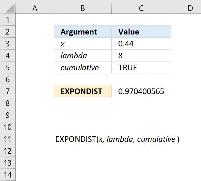
What is the EXPONDIST function?
The EXPONDIST function calculates the exponential distribution representing an outcome in the form of probability.
This function is in the compatibility category and has been replaced by the EXPON.DIST function which was introduced in Excel 2010.
What is an exponential distribution?
The exponential distribution is a continuous probability distribution that models the time between events in a Poisson point process. It is characterized by a constant hazard rate so that the conditional probability of an event does not depend on how much time has passed already.
What is a hazard rate?
The hazard rate is the conditional probability that an event will occur in a small interval given it has not yet occurred. It is often assumed constant in Poisson processes and given by the exponential distribution's parameter.
What is a Poisson point process?
A Poisson point process is a random collection of points representing events in time or space that follow a Poisson distribution. It has independence between points and a constant rate of average occurrence over any interval.
What is a Poisson distribution?
The Poisson distribution is a discrete probability distribution that models the number of events occurring in a fixed interval of time or space. The events must be independent and their average rate is known and constant.
What is independence between points?
Independence between points means that the position or timing of one point in a stochastic spatial or temporal point process does not affect or influence the probability distribution governing the other points. In other words, it is completely random.
What is a stochastic spatial process?
A stochastic spatial process is a random mechanism for generating points distributed in space according to some probability distribution and spatial relationship between the points.
What is a temporal point process?
A temporal point process generates random events in time such as the arrival of customers or radioactive decay with certain probabilistic properties concerning the timing and intervals between events.
What is memorylessness?
Memorylessness is the property of certain probability distributions like the exponential and geometric where past outcomes do not affect future ones, so the conditional probability stays constant regardless of history.
What is a probability distribution?
A probability distribution lets you analyze how likely different random values occurs, in other words, it shows how often we would expect to see different potential values.
What is a continuous probability distribution?
A continuous probability distribution is defined over an interval and range of continuous values, giving the probability an outcome is exactly equal to any value, and having an area under its probability density curve equal to 1.
10.1. Syntax
EXPONDIST(x,lambda,cumulative)
10.2. Arguments
| x | Required. |
| lambda | Required. |
| cumulative | Required. A boolean value. TRUE - cumulative distribution function FALSE - probability density function |
10.3. Example
Formula in cell C7:
10.4. Function not working
The EXPONDIST function returns
- #VALUE! error value if lambda or x is non-numeric.
- #NUM! error value if:
- x < 0 (zero)
- lambda <= 0 (zero)
10.5. How is the EXPONDIST Function calculated?
The general equation to calculate the cumulative distribution function:
The general equation to calculate the probability density distribution:
11. How to use the FDIST function
What is the FDIST function?
The FDIST function calculates the F probability of the right-tailed distribution for two tests. The F.DIST function lets you find out if the means between two given populations are significantly different.
What is the F probability?
The F-distribution or F-ratio is a continuous probability distribution that compare the variances of two populations.
What is variance?
The variance shows how much a set of numbers are spread out from their average value.
Σ(x- x̄)2/(n-1)
x̄ is the sample mean
n is the sample size.
What is a null distribution?
The null hypothesis in the F-distribution is that two independent normal variances are equal. If the observed ratio is too large or too small, then the null hypothesis is rejected, and we conclude that the variances are not equal.
When is a f-distribution used?
The F-distribution is used in the F-test in analysis of variance comparing two variances, as the distribution of the ratio of sample variances when the null is true of no difference between population variances.
What is a continuous probability distribution?
A continuous probability distribution is defined over an interval and range of continuous values, giving the probability an outcome is exactly equal to any value, and having an area under its probability density curve equal to 1.
What are the differences between the F.DIST function and the F.DIST.RT function?
The F.DIST function gives the left-tail area under the curve, while the F.DIST.RT function gives the right-tail area under the curve.
The F.DIST function calculates the cumulative distribution function for the F-distribution, which means it returns the probability that a random variable with an F-distribution is less than or equal to the input F-value.
The F.DIST.RT function calculates the right-tailed probability of the F-distribution, which means it returns the probability that a random variable with an F-distribution is greater than the input F-value.
F.DIST.RT(x, deg_freedom1, deg_freedom2)
F.DIST(x, deg_freedom1, deg_freedom2, cumulative)
11.1 Syntax
FDIST(x, deg_freedom1, deg_freedom2)
11.2 Arguments
| x | Required. |
| deg_freedom1 | Required. Degrees of freedom (numerator). |
| deg_freedom2 | Required. Degrees of freedom (denominator). |
What are the degrees of freedom?
The degrees of freedom parameters are the numerator and denominator chi-squared distributions. They form the ratio that follows the F-distribution.
The degrees of freedom parameters affect the shape of the F-distribution curve and probability, they relate to the samples and capture the amount of information in the variance estimates.
What is a chi-squared distribution?
A chi-squared distribution is a type of probability distribution that is used in statistical tests that compare the variances of two populations. The chi-squared distribution has one parameter, called degrees of freedom, that determines its shape and location. The degrees of freedom represent the number of independent pieces of information used to estimate the variances.
11.3. Example
Formula in cell C7:
11.4. Function not working
The FDIST function returns
- #VALUE! error value if any argument is non-numeric.
- #NUM! error value if:
- x < 0 (zero)
- deg_freedom1 < 1
- deg_freedom1 >= 10^10
- deg_freedom2 < 1
- deg_freedom1 >= 10^10
deg_freedom1 and deg_freedom2 will be converted into integers if they are not.
12. How to use the FLOOR function
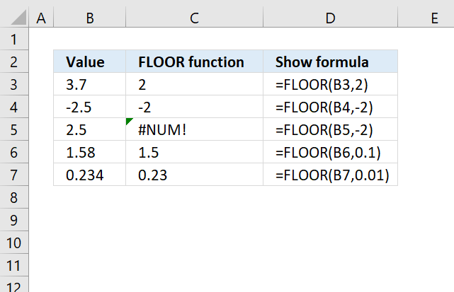
What is the FLOOR function?
The FLOOR function rounds a number down, toward zero, to the nearest multiple of significance.
The function has been replaced by the FLOOR.PRECISE and FLOOR.MATH functions, although it still exists for compatibility with earlier Excel versions.
The FLOOR function may be removed in a future Excel version, use only for backwards compatibility in older software and workbooks.
What is rounding a number?
Rounding is a method to simplify a number by reducing its digits while keeping its approximate value close to the original value.
There are a few common ways to round:
- Round to a set number of decimal places, rounding 2.13579 to 2 decimal places gives 2.14.
- Round up or down to the nearest integer, rounding up 2.3 gives 3. Rounding down 2.3 gives 2.
- Round to a set increment, rounding to the nearest 10 rounds 17 to 20.
- Round to significant figures, rounding 2.333 to 3 significant figures gives 2.33.
When rounding, look at the first digit after where you want to round. If it's 5 or more, round up. If less than 5, round down. Rounding makes numbers cleaner and easier to work with in many everyday situations, however, they may also cause rounding errors like rounded values can compound errors. Rounding measurements and constants may reduces precision. It is better to round numbers after performing calculations than before.
What is a decimal place?
A decimal place refers to each position held by a digit in a number. The first decimal place is the tenths place (1/10), the second is the hundreds place (1/100) and so on.
What is the nearest multiple of significance?
The nearest multiple of significance means to the closest number that a value gets rounded to for a given level of precision. It is based on the number of significant figures or decimal places desired.
For a certain precision, it is the nearest multiple of a power of 10.
For 2 significant figs, nearest multiples are 10, 100, 1000, etc.
For 3 decimal places, nearest multiples are 0.001, 0.01, 0.1, 1, 10, etc.
Values get rounded to the closest multiple of significance at the desired precision. So if reporting to 2 significant figures, 4874 would round to 4900, since the nearest multiple of significance is 100 at that precision.
If reporting to 3 decimal places, 15.4732 would round to 15.473, since the nearest multiple is 0.001. This helps keep rounding consistent and at an appropriate level of precision when doing math calculations and measurements.
What is an integer?
An integer is a whole number that can be positive, negative, or zero, but not a fraction or decimal.
What other Excel functions round numbers?
| ROUND | Rounds a number to a specified number of digits |
| ROUNDUP | Rounds a number up, away from zero |
| ROUNDDOWN | Rounds a number down, towards zero |
| MROUND | Rounds a number to the nearest multiple of a specified value |
| CEILING | Rounds a number up to its nearest multiple. |
| ODD | Returns number rounded up to the nearest odd integer. |
| EVEN | Rounds a number up to the nearest even whole number. |
| FIXED | Rounds a number to the specified number of decimals, lets you ignore comma separators. |
| FLOOR.PRECISE | Rounds a number down to the nearest integer or nearest multiple of significance. |
| FLOOR.MATH | Rounds a number down to the nearest integer or to the nearest multiple of significance. |
12.1. Syntax
FLOOR(number, significance)
12.2. Arguments
| number | Required. The number you want to round. |
| significance | Required. The multiple to which you want to round. |
- A value is rounded down and adjusted toward zero if the number argument is positive.
- A value is rounded down and adjusted away from zero if the number argument is negative.
- No rounding occurs if number is an exact multiple of significance.
12.3. Example
This example demonstrates how to round numbers using the FLOOR function. The first example shown in row three takes number 3.7 and calculates the nearest multiple of significance based argument significance which is specified to 2. The result is 2.
Formula in cell C3:
The second example uses a negative input value in the first argument number which is -2.5 and the significance argument which is specified to -2. The formula in cell C4 returns -2 which is the nearest multiple of significance of -2.
12.4. Function not working
The FLOOR function returns:
- the #VALUE! error value if either argument is nonnumeric.
- the #NUM! error value if number is positive and significance is negative.
13. How to use the FORECAST function
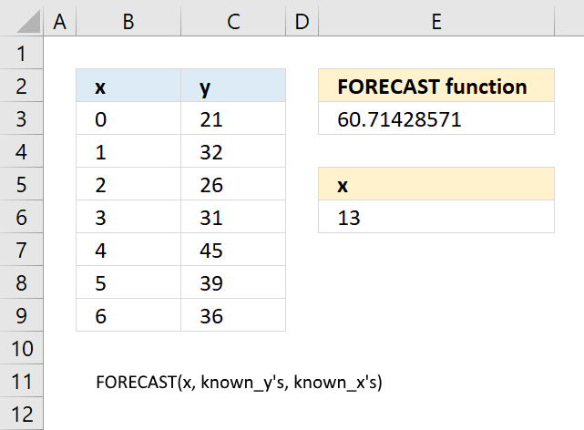
What is the FORECAST function?
The FORECAST function calculates a value based on existing x and y values using linear regression. Use this function to predict linear trends.
There are newer better functions that may have improved accuracy, this function is available for compatibility with older workbooks created in earlier Excel versions and other older software.
This function is outdated and was replaced with FORECAST.LINEAR function in Excel 2016. Microsoft informs that the FORECAST function may not be available in future Excel versions and recommends using the FORECAST.LINEAR function from now on.
What is linear regression?
Linear regression is a statistical technique used to model the linear relationship between a dependent variable and one or more independent variables.
It fits a straight line through the set of data points in such a way that the sum of squared residuals (error) between the line and the points is minimized.
The line equation is defined as Y = a + bx.
Where Y is the dependent variable
x is the independent variable
b is the slope of the line
a is the y-intercept
Regression analysis generates the slope, intercept, and ultimately the line equation that models the relationship between the variables.
What is the slope?
The slope (b) represents the change in Y associated with a unit change in x. Excel lets you calculate the slope with the SLOPE function.
What is the intercept?
The y-intercept (a) is where the line crosses the y-axis when x=0. Excel lets you calculate the intercept with the INTERCEPT function.
What is the R-squared?
R-squared (R2) represents how well the line fits the data. The closer to 1, the better the regression line fits the data. The LINEST function lets you calculate the R-squared value based on known y and known x.
Other ways to calculate the linear regression?

Excel lets you add the linear equation and the line if you plot the data on a scatter chart, simply press with left mouse button on the plus button located on the upper right corner next to the chart. You must select the chart to see the plus button.
Press with left mouse button on the arrow next to the trendline and then press with left mouse button on "Linear Forecast". Double press with left mouse button on the dotted line on the chart to see the settings pane. Press with left mouse button on the checkboxes "Display the equation the chart" and the "Display the R-squared value on the chart" to show the linear regression data on the chart.
What is a linear equation?
A linear equation is a type of equation that can be written in the form ax + b = 0, where a and b are constants and x is a variable. A linear equation represents a relationship between two quantities that are proportional to each other.
For example, if you have a linear equation that says y = 3x + 4, it means that for every unit increase in x, the value of y increases by 3 units and when x is zero y is 4.
The graph of a linear equation is always a straight line, a linear equation does not involve powers of variables.
What is the difference between the FORECAST and the FORECAST.LINEAR function?
The FORECAST function is a legacy function available for compatibility with older software.
13.1 Syntax
FORECAST(x, known_y's, known_x's)
13.2 Arguments
| x | Required. The data point for which you want to predict a value. |
| known_y's | Required. Known y points. |
| known_x's | Required. Known x points. |
13.3 Example
Formula in cell E3:
The chart below shows the predicted value as a red dot, based on x and y values represented by the blue dots.
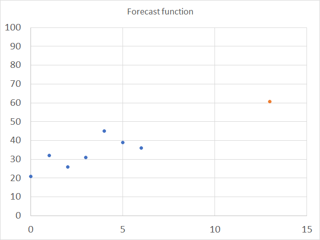
13.4 Function not working
FORECAST function returns a
- #VALUE error if x is not numeric.
- #N/A error if known_y's or known_x's is left out.
- #DIV/0! error value if the variance of known_x's evaluates to zero.
13.5 What is the formula behind the FORECAST function
The mathematical formula behind calculating a simple linear regression is based on minimizing the sum of squared residuals (errors) between the regression line and data points.
Let (x1, y1), (x2, y2), ..., (xn, yn) be the dataset of n points.
The goal is to find the intercept a and slope b for the line equation:
y = a + bx
That minimizes the sum of squared residuals (SSres):
SSres = Σ(yi - ŷi)2
Where ŷi is the predicted y value for point i based on the line. By taking the derivatives of SSres with respect to a and b, setting them equal to 0, and solving, we get:
a = y̅ - b*x̅
b = Σ(xi - x̅)*(yi - y̅) / Σ(xi - x̅)2
Where x̅ and y̅ are the mean values.
This gives the least squares regression line that best fits the data by minimizing the residual sum of squares.
14. How to use the FTEST function
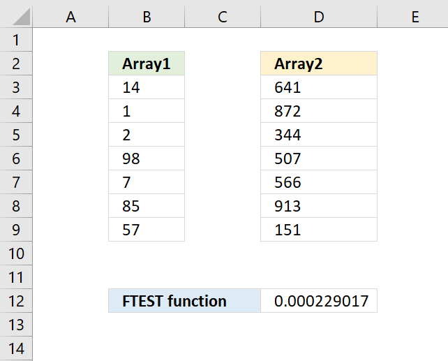
What is the FTEST function?
The FTEST function calculates the value from an F-test. The value shows if the variances from two data sets are not significantly different.
What is the two-tailed probability from an F-test?
The two-tailed probability from an F-test refers to testing against the alternative hypothesis that the two population variances are not equal without specifying direction.
The F-test compares two sample variances by forming a ratio that follows an F-distribution. It tests the null hypothesis that the population variances are equal.
If the variances are not equal which can occur in either direction meaning one could be larger or smaller. A two-tailed test checks both flanks of the F distribution for the probability that the ratio is quite large or quite small. The two-tailed p-value is the total area in both tails combined.
What is a hypothesis in statistics?
In statistics, a hypothesis is an assumption about some aspect of a population or underlying probability model. Hypotheses are of two main types:
- Null hypothesis (H0) - Represents the status quo. Asserts there is no meaningful effect, relationship, or difference in the parameter of interest between groups.
- Alternative hypothesis (H1) - Asserts there is a statistically significant effect in the parameter. Reflects a potential research finding or relationship.
A statistical hypotheses state an assumption that can be tested to reach conclusions from experimental data using methods like t-tests, ANOVA, or chi-square tests.
What is the F probability?
The F-distribution or F-ratio is a continuous probability distribution that compare the variances of two populations.
What is variance?
The variance shows how much a set of numbers are spread out from their average value.
Σ(x- x̄)2/(n-1)
x̄ is the sample mean
n is the sample size.
What is a null distribution?
The null hypothesis in the F-distribution is that two independent normal variances are equal. If the observed ratio is too large or too small, then the null hypothesis is rejected, and we conclude that the variances are not equal.
When is a f-distribution used?
The F-distribution is used in the F-test in analysis of variance comparing two variances, as the distribution of the ratio of sample variances when the null is true of no difference between population variances.
What is a continuous probability distribution?
A continuous probability distribution is defined over an interval and range of continuous values, giving the probability an outcome is exactly equal to any value, and having an area under its probability density curve equal to 1.
14.1 Syntax
FTEST(array1, array2)
14.2 Arguments
| array1 | Required. The first data set. |
| array2 | Required. The second data set. |
14.3 Example
Formula in cell D12:
14.4 Function not working
The arguments must contain numbers or cell references to numbers.
Text, boolean and empty values are ignored.
The FTEST function returns
- #DIV/0! error value if the number of items in each data set don't match.
- #VALUE! error value if any argument is non-numeric.
14.5 How to calculate F statistics?
The LINEST function calculates the F statistic whereas the FTEST function calculates the probability.
14.6 How to calculate the Ftest using an Excel add-in
15. How to use the GAMMADIST function
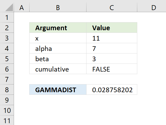
What is the GAMMADIST function?
The GAMMADIST function calculates the gamma often used in queuing analysis in probability statistics.
What is a gamma distribution?
The gamma distribution is a two-parameter continuous probability distribution defined for positive values. It generalizes other distributions like chi-square and exponential and models positively skewed data like time durations.
What is queuing analysis in probability statistics?
Queuing analysis involves using probability and statistics to analyze and model queues (waiting lines). Studies arrival patterns, service times, queue capacity to describe performance and uses probability distributions like Poisson and exponential distributions. It calculates key metrics like expected wait times, queue lengths, utilization.
What is a skewed distribution?
Skewness and asymmetric tails describe the lack of balance and symmetry in probability distributions and datasets. Identifying skewness is fundamental in statistics.
Positive skewness implies a group of values with an asymmetric tail moving toward more positive values. Negative skewness implies a group of values with an asymmetric tail moving toward more negative values.
What is an asymmetric tail?
A symmetric distribution like the normal distribution has no skewness. An asymmetric tail is when one tail of the distribution extends further than the other.
15.1 Example
Formula in cell C7:
15.2 Syntax
GAMMADIST(x,alpha,beta,cumulative)
15.3 Arguments
| x | Required. |
| alpha | Required. |
| beta | Required. 1 returns the standard gamma distribution. |
| cumulative | Required. A boolean value. TRUE - cumulative distribution function FALSE - probability density function |
What is a density function?
A density function in statistics describes the relative likelihood that a random variable takes on a given value. The area under the entire density function integrates to 1.
There are two main types of density functions:
- Probability Density Function (PDF)
PDFs are used for continuous random variables and provides the probability that the variable's value lies within a small range around x.
The area under PDF over an interval provides the probability that the variable lies within that interval. - Probability Mass Function (PMF)
PMFs are used for discrete random variables and gives the exact probability that a variable takes on a specific value x.
15.4 Function not working
The GAMMADIST function returns
- #VALUE! error value if alpha, beta or x is non-numeric.
- #NUM! error value if:
- x < 0 (zero)
- alpha <= 0 (zero)
- beta <= 0 (zero)
15.5 How is the GAMMADIST function calculated?
The equation to calculate the gamma probabiltiy density function:
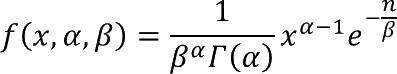
The standard gamma probability function:

16. How to use the LOGNORMDIST function
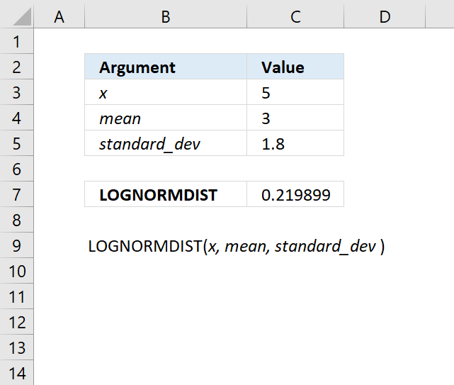
What is the LOGNORMDIST function?
The LOGNORMDIST function calculates the cumulative lognormal distribution of argument x, based on a normally distributed ln(x) with the arguments of mean and standard_dev.
What is the lognormal distribution?
The lognormal distribution is a continuous probability distribution of a random variable whose logarithm follows a normal distribution. It is often used to model a steady relative growth rate is steady like financial returns.
What is a normally distributed ln(x)?
For a random variable x that follows a lognormal distribution like ln(x) is normally distributed. This means that if you take the natural logarithm of x the result will follow a standard normal distribution.
What is a continuous probability distribution?
A continuous probability distribution is defined over an interval and range of continuous values. This gives the probability an outcome that is exactly equal to any value, and having an area under its probability density curve equal to 1.
What is a continuous value?
A continuous value comes from a continuum of possible points rather than distinct separate values. It is able to take on any quantity within an interval rather than certain fixed outcomes.
16.1 Example
Formula in cell C7:
16.2 Syntax
LOGNORMDIST(x, mean, standard_dev)
16.3 Arguments
| x | Required. |
| mean | Required. A value representing the mean of ln(x). |
| standard_dev | Required. A value representing the standard deviation of ln(x). |
What is the mean?
The arithmetic mean is calculated by dividing the sum of all values by the number of values.
For example, an array contains these values: 3,2,1
The sum is 3 + 2 + 1 equals 6
The number of values is 3.
6/3 equals 2. The average of 3, 2, 1 is 2
What is the standard deviation?

Standard deviation tells you how far from the average values are spread out. Both charts above have numbers and an average plotted, they share the same average however, the numbers are not the same.
Chart A above shows that the values are more spread out than the values in chart B. Chart A has a standard deviation of 23.45256334, standard deviation for chart B is 5.207075606. Standard deviation is used in statistics.
What is the cumulative distribution function?
The cumulative distribution function defines the probability that a random variable is less than or equal to a specified value. It gives the area under the probability density curve up to that value.
What is the probability density function?
A probability density function defines a continuous probability distribution by providing the relative likelihood that a random variable takes on different values. The total area under the curve over all values equal to 1.
16.4 Function not working
The LOGNORMDIST function returns
- #VALUE! error value if any argument is non-numeric.
- #NUM! error value if:
- x <= 0
- standard_dev <= 0
16.5 How is the LOGNORMDIST Function calculated?
The equation to calculate the lognormal cumulative distribution is:

17. How to use the MODE function
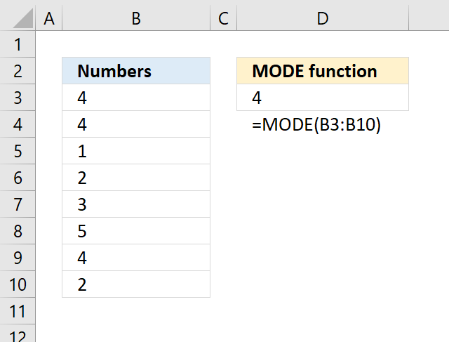
The MODE function calculates the most frequent number in a cell range.
Number 4 exists 3 times on picture above and number 2 exists only 2 times. Number 4 is the most frequent number in B3:B10.
17.1 Syntax
MODE(number1,[number2],...)
17.2 Arguments
| number1 | Required. A cell range you want to calculate the most frequent number. |
| [number2] | Optional. Up to 254 additional arguments. |
17.3 How to get the most common text value

Formula in cell D3:
Explaining formula in cell D3
Step 1 - Create a number representing the position of each value in a sorted array
The COUNTIF function calculates the number of cells equal to a condition. In this case, the less than character compares all values and assigns a number to each value based on their position in a sorted array.
COUNTIF(range, criteria)
COUNTIF(B3:B12, "<"&B3:B12)
becomes
COUNTIF({"Emphasis"; "Basil"; "Boolean"; "Emphasis"; "Gift"; "Historian"; "Boolean"; "Pension"; "Emphasis"; "Yogurt"},"<"&{"Emphasis"; "Basil"; "Boolean"; "Emphasis"; "Gift"; "Historian"; "Boolean"; "Pension"; "Emphasis"; "Yogurt"})
and returns
{3; 0; 1; 3; 6; 7; 1; 8; 3; 9}
Repeated values have identical numbers, we can use this to extract the most common number, see next step.
For example, "Boolean" is displayed twice in B3:B12, shown in the image above. The corresponding number in the array is 1, 1 is shown twice in the array.
Step 2 - Get the most repeated number
The MODE function returns the most common number in a cell range or array.
MODE(COUNTIF(B3:B12, "<"&B3:B12))
becomes
MODE({3; 0; 1; 3; 6; 7; 1; 8; 3; 9})
and returns 3. Number three is the most common number in the array.
Step 3 - Find the position of most repeated number
The MATCH function returns the relative position of an item in an array or cell reference that matches a specified value in a specific order.
MATCH(lookup_value, lookup_array, [match_type])
MATCH(MODE(COUNTIF(B3:B12, "<"&B3:B12)), COUNTIF(B3:B12, "<"&B3:B12), 0)
becomes
MATCH(3, COUNTIF(B3:B12, "<"&B3:B12), 0)
becomes
MATCH(3, {3; 0; 1; 3; 6; 7; 1; 8; 3; 9}, 0)
and returns 1. Three is the first value in the array.
Step 4 - Get value based on position
The INDEX function returns a value from a cell range, you specify which value based on a row and column number.
INDEX(array, [row_num], [column_num], [area_num])
INDEX(B3:B12, MATCH(MODE(COUNTIF(B3:B12, "<"&B3:B12)), COUNTIF(B3:B12, "<"&B3:B12), 0))
becomes
INDEX(B3:B12, 1)
becomes
INDEX({"Emphasis"; "Basil"; "Boolean"; "Emphasis"; "Gift"; "Historian"; "Boolean"; "Pension"; "Emphasis"; "Yogurt"}, 1)
and returns "Emphasis".
17.4 How to get the most common text value - Excel 365
Formula in cell D3:
Explaining formula in cell D3
Step 1 - Count how many times each value is repeated in the array
The COUNTIF function calculates the number of cells equal to a condition.
COUNTIF(range, criteria)
COUNTIF(B3:B12,B3:B12)
becomes
COUNTIF({"Emphasis"; "Basil"; "Boolean"; "Emphasis"; "Gift"; "Historian"; "Boolean"; "Pension"; "Emphasis"; "Yogurt"}, {"Emphasis"; "Basil"; "Boolean"; "Emphasis"; "Gift"; "Historian"; "Boolean"; "Pension"; "Emphasis"; "Yogurt"})
and returns {3; 1; 2; 3; 1; 1; 2; 1; 3; 1}.
Step 2 - Find the largest value
The MAX function returns the largest number in a cell range or array.
MAX(COUNTIF(B3:B12,B3:B12))
becomes
MAX({3; 1; 2; 3; 1; 1; 2; 1; 3; 1})
and returns 3.
Step 3 - Calculate the position of the largest value in array
The equal sign lets you compare value to value, it returns boolean values TRUE or FALSE.
MAX(COUNTIF(B3:B12,B3:B12))=COUNTIF(B3:B12,B3:B12)
becomes
3=COUNTIF(B3:B12, B3:B12)
becomes
3={3; 1; 2; 3; 1; 1; 2; 1; 3; 1}
and returns {TRUE; FALSE; FALSE; TRUE; FALSE; FALSE; FALSE; FALSE; TRUE; FALSE}.
Step 4 - Filter corresponding value
The FILTER function extract values/rows based on a condition or criteria.
FILTER(array, include, [if_empty])
FILTER(B3:B12, MAX(COUNTIF(B3:B12,B3:B12))=COUNTIF(B3:B12,B3:B12))
becomes
FILTER(B3:B12, {TRUE; FALSE; FALSE; TRUE; FALSE; FALSE; FALSE; FALSE; TRUE; FALSE})
becomes
FILTER({"Emphasis"; "Basil"; "Boolean"; "Emphasis"; "Gift"; "Historian"; "Boolean"; "Pension"; "Emphasis"; "Yogurt"}, {TRUE; FALSE; FALSE; TRUE; FALSE; FALSE; FALSE; FALSE; TRUE; FALSE})
and returns {"Emphasis"; "Emphasis"; "Emphasis"}.
Step 5 - Extract unique distinct values
The UNIQUE function extracts both unique and unique distinct values and also compares columns to columns or rows to rows.
UNIQUE(array, [by_col], [exactly_once])
UNIQUE(FILTER(B3:B12, MAX(COUNTIF(B3:B12,B3:B12))=COUNTIF(B3:B12,B3:B12)))
becomes
UNIQUE({"Emphasis"; "Emphasis"; "Emphasis"})
and returns "Emphasis".
Step 6 - Shorten formula
The LET function lets you name intermediate calculation results which can shorten formulas considerably and improve performance.
LET(name1, name_value1, calculation_or_name2, [name_value2, calculation_or_name3...])
The following formula can be shortened using the LET function, cell range B3:B12 is repeated many times in the formula.
Function COUNTIF(B3:B12,B3:B12) is also repeated in the formula, I have assigned z to B3:B12 and y to COUNTIF(B3:B12, B3:B12).
UNIQUE(FILTER(B3:B12, MAX(COUNTIF(B3:B12,B3:B12))=COUNTIF(B3:B12,B3:B12)))
becomes
LET(z, B3:B12, y, COUNTIF(z, z), UNIQUE(FILTER(z, MAX(y)=y)))
18. How to use the PERCENTRANK function
The PERCENTRANK function calculates the percent rank of a given number compared to the whole data set.
What is the percent rank?
The percent rank (or percentile rank) indicates the percentage of scores that fall at or below a given score in a dataset. It provides a way to evaluate the standing of a score relative to others.
What is relative standing?
Relative standing refers to how a particular score compares to the distribution of scores within a group or population. It allows you to understand where a score ranks in relation to others.
When is the PERCENTRANK function useful?
Use the PERCENTRANK.EXC function to evaluate the standing of an aptitude test score among all scores for the test.
What is an aptitude test score?
An aptitude test is a standardized test designed to measure a person's ability or skills in a specific topic. An aptitude test score is the performance measurement on such a test.
Evaluating an aptitude test score's percentage ranking allows understanding its standing compared to other test takers. Higher percentiles indicate better relative performance on the aptitude test.
18.1 Syntax
PERCENTRANK(array, x, [significance])
18.2 Arguments
| array | Required. The array or range of data with numeric values that defines relative standing. |
| x | Required. The value for which you want to know the percent rank. |
| [significance] | Optional. Lower bound, default value 0 (zero). |
What are significant digits?
The PERCENTRANK function does not round the output number to the specified number of significant digits. If the specified number is 3 then 0.1875 becomes 0.187 which means that the remaining digits are simply removed.
18.3 Example
The image above shows 15 numbers in column B. The formula calculates the percent rank for number 11.
Formula in cell C7:
2 numbers are less than 11 (second argument) and 12 numbers are larger than 11.
2/(2+12) = 0.142 (approx 3 digits)
What is percent?
A percent represents a fraction or ratio with a denominator of 100. The term comes from "per cent" meaning out of 100.
A percent expresses a number as a fraction of 100. Converting a fraction or decimal to a percentage involves multiplying by 100 and adding a % symbol. For example, 30% means 30/100 or 0.3. A percentage represents the relative proportion of some quantity compared to 100 units of that quantity
Percentages range between 0% to 100%. 0% means none while 100% means the total amount. They allow standardized measurement of ratios and comparison of part-to-whole relationships. Used frequently in statistics, business, banking, science and other areas involving relative amounts.
What if the x value is not in the array?
The PERCENTRANK function interpolates in order to return the correct value if x doesn't match a value in the array.
What is interpolate?
Interpolate means to estimate or infer a data point within a range of known data points. In statistics, interpolation refers to estimating the percentage between existing data points in a distribution.
18.4 Function not working
The PERCENTRANK function returns
- #NUM! error value if:
- array is empty
- [significance] < 1
19. How to use the QUARTILE function
What is the QUARTILE function?
The QUARTILE function returns the quartile of a data set, use the QUARTILE function to divide data into groups.
What is a quartile?
A quartile is a type of quantile which splits a dataset into four equal parts. The quartiles divide a rank-ordered dataset into four quarters.
There are three quartile values - Q1, Q2, and Q3:
Q1 (first quartile) - 25th percentile
Q2 (second quartile) - 50th percentile (median)
Q3 (third quartile) - 75th percentile
What is the interquartile range (IQR)?
The interquartile range (IQR) is the difference between Q3 and Q1. It indicates the middle 50% spread of the data.
When is it useful to calculate the quartiles?
Quartiles provide quantile-based partitioning of data that reveals distribution, spread, skewness, and outliers. They serve as an important basic statistical summary.
What is quantile?
Quantiles are a statistical technique for dividing a dataset into equal-sized groups for analysis. Quantiles split data into equal-sized subsets when ordered from smallest to largest.
The quartiles, percentiles, quintiles, deciles, etc. are examples of quantiles.
- Quartiles split data into 4 equal groups
- Percentiles into 100 groups,
- Quintiles into 5.
Quantiles can show aspects of shape, spread, and concentration.
How to graph quartiles?
The Box and Whisker chart display quartiles.
19.1 Syntax
QUARTILE(array, quart)
19.2 Arguments
| array | Required.The cell values for which you want to calculate the quartile value. |
| quart | Required. Indicates which value to return, see table below. |
| Quart parameters | |
|---|---|
| 0 | Minimum value. |
| 1 | First quartile (25th percentile). |
| 2 | Median quartile (50th percentile). |
| 3 | Third quartile (75th percentile). |
| 4 | Maximum value. |
19.3 Example
This example demonstrates the QUARTILE function, the image above shows the following values in B3:B11: 66, 97, 99, 77, 9, 60, 35, 60, 61
Formula in cell D3:
Here is how the QUARTILE function calculates the first Quartile (Q1). The median is 61 based on the numbers in cell range B3:B11. The first half contains the following numbers: 9, 35, 61, 60, and 60 The median of these numbers is 60.
The QUARTILE function returns the same value as:
- MIN function if quart is 0 (zero)
- MEDIAN function if quart is 2.
- MAX function if quart is 4
What is the MEDIAN?
The median value is the middle number of a group of numbers when arranged from smallest to largest. It returns a good measure of the typical value in a data set that is not affected by outliers or skewness . For example, the median income may be a better measure of the average income than the mean. The mean can be distorted by a few very high incomes which is the case, for instance, in the US. The very high incomes represent the outliers.
For example, a group containing an odd number of values like five numbers: 1, 3,4,9, and 11 has the middle value 4. 1 and 3 are smaller and 9 and 11 are larger.
A group containing an even number of values like: 1,3,9, and 11 has a median of 6. There are two middle numbers in the group which are 3 and 9. 3 + 9 = 12 and 12/2 equals 6.
What is the MIN function?
The MIN function returns the smallest number in a cell range.
Function syntax: MIN(number1, [number2], ...)
What is the MEDIAN function?
The MEDIAN function calculates the median based on a group of numbers. The median is the middle number of a group of numbers.
Function syntax: MEDIAN(number1, [number2], ...)
What is the MAX function?
The MAX function calculate the largest number in a cell range.
Function syntax: MAX(number1, [number2], ...)
19.4 Function not working
The QUARTILE function returns #NUM! value if
- quart < 0 (zero)
- quart > 4
19.5 How is the QUARTILE function calculated?
QUARTILE function calculates quartiles using the inclusive method:
Data is sorted lowest to highest. The quartile boundaries include the quartile values themselves.
For example, for the data {1, 2, 3, 4, 5}:
Q0 = 1
Q1 = 2
Q2 = 3
Q3 = 4
The median of data {1, 2, 3, 4, 5} is 3. The first half contains 1 , 2, and 3. The median of 1,2, and 3 is 2 = Q1
Q2 is the median: 3
The second half contains 3, 4 and 5, The median of 3, 4 and 5 is 4 = Q3
20. How to use the RANK function
![]()
What is the RANK function?
The RANK function calculates the size of a specific number compared to a list of numbers. It allows you to rank numbers relative to their sizes in ascending or descending order.
There are newer better functions that may have improved accuracy, this function is available for compatibility with Excel 2007 and earlier versions.
This function is outdated and was replaced with RANK.AVG function and the RANK.EQ function. The RANK function may not be available in future Excel versions and Microsoft recommends using the newer functions from now on.
What are the differences between the RANK, RANK.EQ and RANK.AVG functions?
First, the RANK function is a legacy function and should be avoided if possible. The RANK.EQ function and the RANK function rank numbers based on size, however, they share the rank if two or more numbers are equal. For example:
| Numbers | RANK.EQ | RANK |
| 10 | 4 | 4 |
| 20 | 2 | 2 |
| 20 | 2 | 2 |
| 30 | 1 | 1 |
The RANK.AVG function returns the rank of a number in a list of numbers. If more than one value share the same rank, the average rank is returned. For example:
| Numbers | RANK.AVG |
| 10 | 4 |
| 20 | 2.5 |
| 20 | 2.5 |
| 30 | 1 |
What are the differences between the RANK and PERCENTRANK functions?
The PERCENTRANK function calculates the percent rank of a given number compared to the whole data set.
| Numbers | RANK | PERCENTRANK |
| 10 | 4 | 0 |
| 20 | 2.5 | 0.333 |
| 20 | 2.5 | 0.333 |
| 30 | 1 | 1 |
The PERCENTRANK function is also a legacy function and should be avoided if possible. Use the PERCENTRANK.EXC or the PERCENTRANK.INC.
Other ways to rank numbers in a list?
![]()
Data Bars is a conditional formatting feature that allows you to create horizontal bars that represent a corresponding number. This allows you to more quickly scan a group of numbers for the largest and smallest numbers.
![]()
Color scales is also a conditional formatting feature that allows you to highlight cells based on the size of their numbers.
Why is ranking numbers useful in statistics?
Ranking numbers in statistics refers to converting data values into their ranked order.
- Reduces the impact of outliers
Extreme values don't distort ranks as much as raw scores. - Easier to interpret
Ranks provide a sense of relative standing on a consistent scale from lowest to highest. - Allows non-parametric tests
Statistical tests that don't rely on parameterized distributions. - Simplifies combining scores
Ranks provide a common scale for scores from different sources. - Assesses relative performance
Ranks indicate how a value compares to others in the dataset. - Analyze changes in rank
Shifts in ranks over time can be meaningful even if values don't change much. - Identify top/bottom performers
Ranks make it easy to find top and bottom values. - Tied ranks for equal values
Accounts for duplicate values getting the same mean rank.
20.1 Syntax
RANK(number,ref,[order])
20.2 Arguments
| number | Required. The number you want to calculate the rank for. |
| Ref | Required. An array or cell reference to a list of numerical values. |
| Order | Optional. How to rank the number, 1 - ascending or 0 - descending. If omitted - descending order. |
What is ascending?
Ascending is a term used to describe the order and sequence of data. Ascending order sorts data from lowest to highest.
Arranging data points from lowest to highest value. Also known as increasing order. The ranking goes up, with smaller values first.
Example: Sorting numbers 1, 2, 3 in ascending order.
What is descending?
Descending is a term used to describe the order and sequence of data. Descending order sorts data from highest to lowest.
Arranging data points from highest to lowest value, also known as decreasing order. The ranking goes down, with larger values first.
Example: Sorting numbers 3, 2, 1 in descending order.
20.3 example
![]()
The image above shows 5 digit numbers in cell range B3:B15, the corresponding cells on the same row in column C shows the rank output from the RANK function. The RANK function returns a number representing the position if they were sorted in ascending or descending order.
Formula in cell C3:
The largest number is in cell B15, cell C15 contains the output from the RANK function which is 1. The smallest number is in cell B12, cell C12 shows 13 which is the rank. There are 13 numbers in cell range B3:B15 and the rank 13 tells us that the number is the smallest based on it's size compared to the other numbers in the list.
![]()
20.4 Alternative
![]()
The COUNTIF function allows you to count cells based on a condition. The smaller than or larger than character lets you count numbers that are smaller or larger respectively.
Formula in cell C3:
The COUNTIF function calculates the number of cells that is equal to a condition.
Function syntax: COUNTIF(range, criteria)
For example, cell range B3:B15 contains five numbers larger than the number in cell C3. The COUNTIF function returns five indicating that the number in cell B3 is the sixth largest number, the reason why is because the COUNTIF function returns 0 (zero) for the largest number in the group. One for the second largest and so on.
To make the COUNTIF function return the same number as the RANK function then add 1 to the function like this:
Why is the COUNTIF function returning 0 (zero) for the largest number in a list?
The COUNTIF function counts the number of cells that contain a number larger than the condition.
For example, there is no number larger than the largest number and that makes the COUNTIF function return 0 (zero).
The COUNTIF function also counts text values, this is demonstrated in the next section below.
20.5 How to rank text
![]()
Did you know that it is possible to rank text strings using the COUNTIF function? It returns a number corresponding to the position in a sorted list except that the top text value starts with 0 (zero).
For example:
A - 0
B - 1
C - 2
D - 3
F - 4
The list above is sorted from A to Z.
Formula in cell C3:
The COUNTIF function is one of the more useful functions in Excel, this is just one example.
Recommended articles

Counts the number of cells that meet a specific condition.
21. How to use the STDEV function

What is the STDEV function?
The STDEV function calculates the standard deviation of a sample of values. The standard deviation shows how much the values differ from the mean value.
There are two different math formulas for calculating the standard deviation, the STDEV function tries estimates the standard deviation based on a sample of values whereas the STDEV.P function calculates the standard deviation based on the entire population.
Section 5 below describes the differences in how the standard deviation is calculated.
There are newer better functions that may have improved accuracy, this function is available for compatibility with older workbooks created in earlier Excel versions and other older software.
The new STDEV.S function replaces the older STDEV function which has better accuracy, Microsoft tells us that the STDEV function may not be available in future Excel versions and recommends us using the STDEV.S from now on.
Table of Contents
21.1. What is Standard Deviation?
Standard deviation tells you how far from the mean values are spread out. Both charts above have numbers and an average plotted, they share the same average however, the numbers are not the same.
Chart A above shows that the values are more spread out than the values in chart B. Standard deviation is used in statistics.
A low standard deviation number near 0 (zero) tells us that the data points are located very close to the mean, a larger standard deviation value indicates data points are more spread out from the mean.
The most commonly used symbol for standard deviation is σ which is the lower case greek letter sigma. σ was chosen because standard deviation is calculated using summation Σ which is the upper case greek letter sigma.
σ is used to represent population standard deviation. s is used to represent sample standard deviation. In statistics formulas, σ is used along with the mean symbol μ to represent a distribution.
What is the mean?
The mean is also called the average. The mean is calculated by adding all the values in a dataset and dividing by the total number of values. Excel has functions for calculating the average. AVERAGE function
For example, a data set contains 5, 2,6,8, and 4. The total is 5 + 2 + 6 + 8 + 4 equals 25. The average is 25 / 5 equals 5.
What is one standard deviation in a normal distribution?

One standard deviation from the mean μ captures 34.13% of the data on each side, or 68.27% total in a standard normal distribution. This percentage allows standard deviations to indicate where values fall in the distribution.
What is two standard deviations in a normal distribution?

Two standard deviations from the mean μ captures 47.5% of the data on each side, or 95% total in a standard normal distribution.
What is three standard deviations in a normal distribution?

Tree standard deviations from the mean μ captures 48.85% of the data on each side, or 97.7% total in a standard normal distribution.
21.2. STDEV Function Syntax
STDEV(number1,[number2],...)
21.3. STDEV Function Arguments
| number1 | Required. This argument can be an array of constants or a cell reference to a group of values. |
| [number2] | Optional. Up to 254 additional arguments. |
21.4. STDEV Function Example
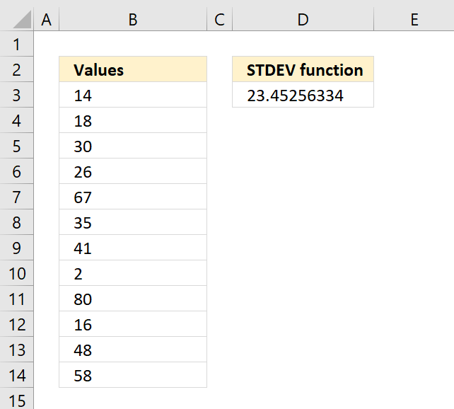
Formula in cell C3:
21.5. How is the STDEV function calculated?
The STDEV function is entered in cell D3, here is how the function calculated the output:

x ̅ is the average.
n is how many values.
Step 1 - Calculate the average
14 + 18 + 30 + 26 + 67 + 35 + 41 + 2 + 80 + 16 + 48 + 58 = 435
435/12 = 36.25
Step 2 - Subtract the average and square the result for all values
(14-36.25)^2 + (18-36.25)^2 + (30-36.25)^2 + (26-36.25)^2 + (67-36.25)^2 + (35-36.25)^2 + (41-36.25)^2 + (2-36.25)^2 + (80-36.25)^2 + (16-36.25)^2 + (48-36.25)^2 + (58-36.25)^2
becomes
(-22.25)^2+(-18.25)^2+(-6.25)^2+(-10.25)^2+(30.75)^2+(-1.25)^2+(4.75)^2+(-34.25)^2+(43.75)^2+(-20.25)^2+(11.75)^2+(21.75)^2
becomes
495.0625+333.0625+39.0625+105.0625+945.5625+1.5625+22.5625+1173.0625+1914.0625+410.0625+138.0625+473.0625
and returns
6050.25
Step 3 - Divide with the total count minus 1
6050.25/11 equals 550.022727272727
Step 4 - Square root the result
550.022727272727^(1/2) equals 23.4525633411942
21.6. What is the difference between the STDEV function and the STEDV.P function?
The STDEV function estimates an output based on a sample of values, the STEDV.P however, calculates the standard deviation based on the entire population of values.
STDEV function formula:
STDEV.P function formula:

These formula differences explain why the functions return different values even if you use the same values.
21.7. What is the difference between the standard deviation and variance?
Standard deviation measures the amount of dispersion around the mean, while variance represents the average squared deviation. Standard deviation provides an interpretable and tangible idea of spread, while variance is a more abstract representation. In general, standard deviation is more widely used and reported than variance, as it's more understandable.
VAR function formula:

STDEV function formula:
The math formulas above demonstrates that standard deviation is the square root of the variance.
Array Manipulation Functions 13 Mar 2024 1:22 AM (2 years ago)
Table of Contents
- How to use the CHOOSECOLS function
- How to use the CHOOSEROWS function
- How to use the DROP function
- How to use the EXPAND function
- How to use the HSTACK function
- How to use the TAKE function
- How to use the TOCOL function
- How to use the TOROW function
- How to use the VSTACK function
- How to use the WRAPCOLS function
- How to use the WRAPROWS function
1. How to use the CHOOSECOLS function

What is the CHOOSECOLS function?
The CHOOSECOLS function returns given columns from a cell range or array.
The image above shows a set of values in cell range B2:D5, I have enetered a CHOOSECOLS formula in cell B9:
It spills values to cells below and to the right of cell B9 as far as needed, this is done automatically. This specific formula in cell B9 extracts columns 2 and three from B2:D5.
The CHOOSECOLS function is available to Excel 365 users and is in the "Array manipulation" category.
Table of Contents
- CHOOSECOLS Function Syntax
- CHOOSECOLS Function Arguments
- CHOOSECOLS Function example
- How to combine specific cell range columns - Excel 365
- How to combine specific columns based on a given value - Excel 365
- How to combine columns using negative values - Excel 365
- CHOOSECOLS function returns a #VALUE! error
- Extract values from given columns and return the list in random order - Excel 365
- Join multiple non-adjacent cell ranges and return given columns (3D range) - Excel 365
- Get Excel file
1.1. CHOOSECOLS Function Syntax
CHOOSECOLS(array, col_num1, [col_num2], …)
1.2. CHOOSECOLS Function Arguments
| array | Required. The source cell range or array. |
| col_num1 | Required. A number represents the column in a given cell range. |
| [col_num2] | Optional. Extra column numbers to be extracted. |
1.3. CHOOSECOLS Function example

The picture above shows how the CHOOSECOLS function extracts the second and third column from cell range B2:D5.
Dynamic array formula in cell B9:
The image contains numbers below each column in cell range B2:D5, the numbers lets you easily identify columns 2 and 3. The output is shown in cell B9, columns 2 and 3 are extracted from B2:D5.
Excel 365 dynamic array formulas are different than regular array formulas. The former are entered as regular formulas, however they automatically spill values below and to the right as far as needed. A #SPILL! error is displayed if a cell is not empty where spilling needs to be returned. Simply delete the value and the formula works again.
1.3.1 Explaining formula
Step 1 - CHOOSECOLS function
The CHOOSECOLS function has two required arguments and one optional. The optional argument is not limited to one value, it can be up to at least 254 arguments.
CHOOSECOLS(array, col_num1, [col_num2], …)
Step 2 - Populate arguments
array - B2:D5
col_num1 - 2
[col_num2] - 3
Step 3 - Evaluate function
CHOOSECOLS(B2:D5, 2, 3)
becomes
CHOOSECOLS({89, 27, 26;
68, 84, 98;
19, 92, 62;
37, 63, 45}, 2, 3)
and returns
{27, 26; 84, 98;
92, 62; 63, 45}
The image below shows the array in cell range B9:C12.
1.4. How to combine specific cell range columns - CHOOSECOLS Function

The CHOOSECOLS function lets you use an array in the arguments, the image above demonstrates a CHOOSECOLS function that uses an array in the second argument. This means that you are not limited to arguments, you can use an array in one argument. This makes it possible to use a lot more than 254 columns.
Dynamic array formula in cell B9:
The image above has values in cell range B2:D5, I have entered blue numbers below each column so you can more easily see the extracted columns. Columns 1 and 3 are returned to a dynamic array that spills values to cells below and to the right as far as needed.
This makes the CHOOSECOLUMNS function useful for combining specific columns from a given data set., this in return makes it even easier to work with arrays in Excel 365 than in earlier Excel versions.
Explaining formula
Step 1 - Populate the array
The curly brackets let you build an array that you can use in most but not all Excel functions. The ; semicolon is a delimiting character that separates values row by row.
The CHOOSE function requires numbers separated with semicolons or whatever row delimiting character you use.
{1; 3}
Step 2 - CHOOSECOLS function
CHOOSECOLS(array, col_num1, [col_num2], …)
CHOOSECOLS(B2:D5, {1; 3})
becomes
CHOOSECOLS({89, 27, 26;
68, 84, 98;
19, 92, 62;
37, 63, 45}, {1; 3})
and returns
{89, 26;
68, 98;
19, 62;
37,45}
1.5. How to combine specific columns based on a given value - CHOOSECOLS Function

The section shows how to return specific columns based on a string containing numbers delimited by a character. The TEXTSPLIT function separates values into an array.
Cell F2 contains the foloowing thext string: 1,2 This string is separated into an array using the comma as a delimiting character. The array is then used to extract columns 1 and 2 from cell range B2:D5.
Dynamic array formula in cell B9:
This is handy if the Excel user needs to specify the given columns in a cell, which in turn makes it more user friendly than editing hard-coded values in a formula. Working with arrays has never been easier, the new Excel 365 functions are very much so appreciated.
Explaining formula
Step 1 - Split text
The TEXTSPLIT function lets you split a string into an array across columns and rows based on delimiting characters.
TEXTSPLIT(Input_Text, col_delimiter, [row_delimiter], [Ignore_Empty])
TEXTSPLIT(F2,,",")
becomes
TEXTSPLIT("1,2", , ",")
and returns {"1"; "2"}.
Note the double quotes, Excel handles these values as text values. The next step converts text values to numbers.
Step 2 - Convert text to numbers
The asterisk lets you multiply numbers in an Excel formula, I am using it here to convert text to numbers.
TEXTSPLIT(F2,,",")*1
becomes
{"1"; "2"}*1
and returns {1; 2}.
Step 3 - CHOOSECOLS function
CHOOSECOLS(B2:D5,TEXTSPLIT(F2,,",")*1)
becomes
CHOOSECOLS(B2:D5, {1; 2})
becomes
CHOOSECOLS({89, 27, 26;
68, 84, 98;
19, 92, 62;
37, 63, 45}, {1; 2})
and returns
{89, 27;
68, 84;
19, 92;
37, 63}
The image below shows the array described above in cell B9, the dynamic array formula spills values cells below and to the right as far as needed.
1.6. How to combine columns using negative values - CHOOSECOLS Function

The CHOOSECOLS function lets you also use negative numbers, this will make the function count columns from right to left.
This is useful if you have a large array containing many columns. If you need to extract columns located to the far right, instead of counting columns from left to right you can use negative integers and count from right to left. This may save you time and less prone to errors.
Formula in cell B9:
CHOOSECOLS(array, col_num1, [col_num2], …)
The image above shows an array in cell range B2:C5. The formula in cell B9 extracts the last column and the next one counting from right to left using negative numbers.
1.7. CHOOSECOLS function returns a #VALUE! error

The CHOOSECOLS function returns a #VALUE! error when no values can be displayed.Here is a scenario when this can happen.
The image above displays an array in cell range B2:D5, the formula in cell B9 tries to extract the fifth column from B2:D5, however, there are only three columns in cell range B2:D5.
This makes it impossible for the CHOOSECOLS function to extract the fifth column thus returning the #VALUE error. You can catch errors using the IFERROR function, however, hiding errors is not always great. The downside is that if hide errors you make them much harder to find. Finding errors is most important in order to troubleshoot and find a solution to the problem.
1.8. Extract values from given columns and return the list in random order - CHOOSECOLS function

The image above shows an array in cell range B2:D5. The formula in cell B8 returns values in random order from columns two and three in B2:D5.
Dynamic array formula in cell B8:
The result in cell B8 shows an array with the same size as column 2 and 3 from cell range B2;D5. However, the values from column 2 and 3 are in random order. Note that the formula also only returns values from column 2 and 3 but in random order.
1.8.1 Explaining formula in cell B8
Step 1 - Filter columns 2 and 3
CHOOSECOLS(B2:D5, 2, 3)
becomes
CHOOSECOLS({89, 27, 26;
68, 84, 98;
19, 92, 62;
37, 63, 45}, 2, 3)
and returns
{27,26;
84,98;
92,62;
63,45}
Step 2 - Rearrange values to a single row
The TOROW function rearranges values from a 2D cell range or array to a single row.
TOROW(array, [ignore], [scan_by_col])
TOROW(CHOOSECOLS(B2:D5,2,3))
becomes
TOROW({27,26;
84,98;
92,62;
63,45}
and returns
{27, 26, 84, 98, 92, 62, 63, 45}.
Step 3 - Count cells
The COLUMNS function returns the number of columns in a given cell range or array.
COLUMNS(array)
COLUMNS(TOROW(CHOOSECOLS(B2:D5,2, 3)))
becomes
COLUMNS({27, 26, 84, 98, 92, 62, 63, 45})
and returns 8.
Step 4 - Count rows
The ROWS function returns the number of rows in a given cell range or array.
ROWS (array)
ROWS(CHOOSECOLS(B2:D5,2, 3))
becomes
ROWS({27,26;
84,98;
92,62;
63,45})
and returns 4.
Step 5 - Create random decimal numbers
The RANDARRAY function returns a table of random numbers across rows and columns.
RANDARRAY([rows], [columns], [min], [max], [whole_number])
RANDARRAY(,COLUMNS(TOROW(CHOOSECOLS(B2:D5,2, 3))))
becomes
RANDARRAY(,6)
and returns
{0.215398134613085, 0.390607168196479, ... ,0.83231474462401}.
Step 6 - Rearrange values in random order
The SORTBY function allows you to sort values from a cell range or array based on a corresponding cell range or array.
SORTBY(array, by_array1, [sort_order1], [by_array2, sort_order2],…)
SORTBY(TOROW(CHOOSECOLS(B2:D5,2, 4)),RANDARRAY(,COLUMNS(CHOOSECOLS(B2:D5,2, 3))))
becomes
SORTBY({27,26;
84,98;
92,62;
63,45}, {0.215398134613085, 0.390607168196479, ... ,0.83231474462401})
and returns
{84, 98, 27, 92, 62, 26, 45, 63}
Step 7 - Rearrange values to the original array size
The WRAPCOLS function rearranges values from a single row to a 2D cell range based on a given number of values per column.
WRAPCOLS(vector, wrap_count, [pad_with])
WRAPCOLS(SORTBY(TOROW(CHOOSECOLS(B2:D5,2, 4)),RANDARRAY(,COLUMNS(TOROW(CHOOSECOLS(B2:D5,2, 4))))),ROWS(CHOOSECOLS(B2:D5,2, 3)))
becomes
WRAPCOLS({63, 37, 45, 98, 84, 68}, ROWS(CHOOSECOLS(B2:D5,2, 3)))
becomes
WRAPCOLS({84, 98, 27, 92, 62, 26, 45, 63}, 4)
and returns
{84, 98; 27, 92; 62, 26; 45, 63}.
Step 8 - Shorten formula
The LET function lets you name intermediate calculation results which can shorten formulas considerably and improve performance.
LET(name1, name_value1, calculation_or_name2, [name_value2, calculation_or_name3...])
WRAPCOLS(SORTBY(TOROW(CHOOSECOLS(B2:D5, 2, 3)), RANDARRAY(, COLUMNS(TOROW(CHOOSECOLS(B2:D5, 2, 3))))), TOROW(CHOOSECOLS(B2:D5, 2, 3)))
becomes
LET(z, CHOOSECOLS(B2:D5, 2, 3), x, TOROW(z), WRAPCOLS(SORTBY(x, RANDARRAY(, COLUMNS(x))), ROWS(z)))
1.9. Join multiple non-adjacent cell ranges and return given columns (3D range) - CHOOSECOLS function

The image above shows three data sets in cell ranges B3:D6, F3:H6, and J3:L6. The formula in cell B9 merges these three non-contiguous cell ranges vertically and returns columns 1 and 2.
Dynamic array formula in cell B9:
This is a rather complicated manipultaion of three different cell ranges. The CHOOSECOLS and VSTACK functions makes it super easy to join the cell ranges and then extract only column 1 and 2.
This formula can be really useful if you want to work with cell ranges across multiple worksheets and apply different calculations, for example, like finding the average or return unique distinct values. These types of calculations have never been easier with the new Array manipulation functions.
1.9.1 Explaining formula
Step 1 - Stack values horizontally
The VSTACK function lets you combine cell ranges or arrays, it joins data to the first blank cell at the bottom of a cell range or array (vertical stacking)
VSTACK(array1, [array2],...)
VSTACK(B3:D6, F3:H6, J3:L6)
becomes
VSTACK({"Peach", 43, 1.03;"Blueberry", 39, 1.48;"Apple", 46, 1.1;"Grapefruit", 14, 0.72}, {"Mandarin", 29, 0.78;"Raspberry", 33, 1.07;"Plum", 25, 0.9;"Mango", 37, 1.13}, {"Pear", 17, 0.63;"Orange", 31, 1.06;"Lime", 17, 1.27;"Kiwi", 45, 0.58})
and returns
{"Peach", 43, 1.03;
"Blueberry", 39, 1.48;
"Apple", 46, 1.1;
"Grapefruit", 14, 0.72;
"Mandarin", 29, 0.78;
"Raspberry", 33, 1.07;
"Plum", 25, 0.9;
"Mango", 37, 1.13;
"Pear", 17, 0.63;
"Orange", 31, 1.06;
"Lime", 17, 1.27;
"Kiwi", 45, 0.58}
Step 2 - Filter given rows
CHOOSECOLS(VSTACK(B3:D6, F3:H6, J3:L6),1, 2)
becomes
CHOOSECOLS({"Peach", 43, 1.03;
"Blueberry", 39, 1.48;
"Apple", 46, 1.1;
"Grapefruit", 14, 0.72;
"Mandarin", 29, 0.78;
"Raspberry", 33, 1.07;
"Plum", 25, 0.9;
"Mango", 37, 1.13;
"Pear", 17, 0.63;
"Orange", 31, 1.06;
"Lime", 17, 1.27;
"Kiwi", 45, 0.58}, 1, 5, 9)
and returns
{"Peach", 43;
"Blueberry", 39;
"Apple", 46;
"Grapefruit", 14;
"Mandarin", 29;
"Raspberry", 33;
"Plum", 25;
"Mango", 37;
"Pear", 17;
"Orange", 31;
"Lime", 17;
"Kiwi", 45}
How to use the CHOOSECOLS functionv2
Useful links
CHOOSECOLS function - Microsoft support
CHOOSECOLS Function in Excel: Explained
CHOOSECOLS function in Excel to get columns from array or range
2. How to use the CHOOSEROWS function

What is the CHOOSEROWS function?
The CHOOSEROWS function returns given rows from a cell range or array.
The CHOOSEROWS function is available to Excel 365 users and is in the "Array manipulation" category.
Table of Contents
- CHOOSEROWS Function Syntax
- CHOOSEROWS Function Arguments
- CHOOSEROWS Function example
- CHOOSEROWS Function example - array
- CHOOSEROWS Function example - split text to array
- CHOOSEROWS Function example - negative values
- CHOOSEROWS Function errors
- CHOOSEROWS Function - values in random order
- CHOOSEROWS Function - multiple source ranges
- Get every other row
- Get Excel file
2.1. CHOOSEROWS Function Syntax
CHOOSEROWS(array, row_num1, [row_num2], …)
2.2. CHOOSEROWS Function Arguments
| array | Required. The source cell range or array. |
| row_num1 | Required. A number representing the row in a given cell range. |
| [row_num2] | Optional. Extra row numbers to be extracted. |
2.3. CHOOSEROWS Function example

The picture above shows how the CHOOSEROWS function extracts the second and fourth row from cell range B2:D5 leaving the first and third row out.
Dynamic array formula in cell B9:
The image above shows values in cell range B2:D5, the formula in cell B9 extracts rows 2 and 4 and merges these rows to a single array. The array has the same number of columns as B2:D5 except that it now only contains two rows.
Excel 365 dynamic array formulas are different than regular array formulas in earlier Excel versions. Excel 365 dynamic array formulas are entered as regular formulas, however they automatically spill values below and to the right as far as needed.
If the destination range is not empty a #SPILL! error is shown. It is easy to fix this problem, delete the value and the Excel 365 formula works again.
2.3.1 Explaining formula
Step 1 - CHOOSEROWS function
CHOOSEROWS(array, row_num1, [row_num2], …)
Step 2 - Populate arguments
array - B2:D5
row_num1 - 2
[row_num2] - 4
Step 3 - Evaluate function
CHOOSEROWS(B2:D5, 2, 4)
becomes
CHOOSEROWS({89, 27, 26;
68, 84, 98;
19, 92, 62;
37, 63, 45}, 2)
and returns
{68, 84, 98;
37, 63, 45}
The returned array is shown in B9:E10 in the image below.
2.4. CHOOSEROWS Function example - array

The CHOOSEROWS function lets you use an array in the arguments, the image above shows an array in the second argument {1;4}. An array begins with a curly bracket { and ends with a curly bracket }. These characters tell Excel that this is an array.
Using an array in an argument lets you specify the rows which you want to keep, the remaining rows are filtered out. This lets you enter rows in one argument only if you prefer.
Values in an array are delimited by one character for rows and one for columns, which you use are determined by your regional settings in windows. My settings use a semicolon for rows and a comma for columns.
Dynamic array formula in cell B9:
This example demonstrates values in cell range B2:D5, displayed in the image above. The formula in cell B9 returns an array containing rows 1 and 4, the number of columns match the original array B2:D5. Use the CHOOSECOLS function when you want to resize an array based on rows, for example, if you want to calculate the median or frequency based on a particular row or rows in an array.
This was very difficult in earlier versions, Excel 365 is a big step forward. Excel 365 spills values to cell B9 and cells below and to the right as far as needed. A #SPILL error is shown if a cell contains a value. Delete the value so the formula can show all values in the array.
Explaining formula
Step 1 - Populate the array
The curly brackets let you build an array that you can use in most but not all Excel functions. The ; semicolon is a delimiting character that separates values row by row.
The CHOOSE function requires numbers separated with semicolons or whatever row delimiting character you use.
{1; 4}
Step 2 - CHOOSEROWS function
CHOOSEROWS(array, row_num1, [row_num2], …)
CHOOSEROWS(B2:D5, {1; 4})
becomes
CHOOSEROWS({89, 27, 26;
68, 84, 98;
19, 92, 62;
37, 63, 45}, {1; 4})
and returns
{89, 27, 26;
37, 63, 45}
2.5. CHOOSEROWS Function example - split text to array

The section shows how to return specific rows based on a string containing numbers. Cell F2 contains a text value containing numbers delimited by a comma.
The TEXTSPLIT function separates the values in to an array that the CHOOSEROWS function can use to filter the given rows.
Dynamic array formula in cell B9:
The image above shows values in cell range B2:D5, the specified rows is in cell F2. The formula in cell B9 returns rows 1, 3 and 4 to cell B9 based on the specified numbers in cell F2. Excel 365 spills values to cell B9 and cells below and to the right as far as needed.
A #SPILL error is returned if a cell is not empty, this restricts the dynamic array formula to show all values in the array. Simply delete the cell containing the value and the formula works again.
Explaining formula
Step 1 - Split text
The TEXTSPLIT function lets you split a string into an array across columns and rows based on delimiting characters.
TEXTSPLIT(Input_Text, col_delimiter, [row_delimiter], [Ignore_Empty])
TEXTSPLIT(F2,,",")
becomes
TEXTSPLIT("1,3,4",,",")
and returns {"1"; "3"; "4"}. Note the double quotes, Excel handles these values as text values. The next step converts text values to numbers.
Step 2 - Convert text to numbers
The asterisk lets you multiply numbers in an Excel formula, I am using it here to convert text to numbers.
TEXTSPLIT(F2,,",")*1
becomes
{"1"; "3"; "4"}*1
and returns {1; 3; 4}.
Step 3 - CHOOSEROWS function
CHOOSEROWS(B2:D5,TEXTSPLIT(F2,,",")*1)
becomes
CHOOSEROWS(B2:D5, {1; 3; 4})
becomes
CHOOSEROWS({89, 27, 26;
68, 84, 98;
19, 92, 62;
37, 63, 45}, {1; 3; 4})
and returns
{89,27,26;
19,92,62;
37,63,45}
2.6. CHOOSEROWS Function example - negative values

The CHOOSEROWS function lets you use negative numbers, this will make the function count from the bottom or from the end. This is really helpful if you array is large and you want to select rows close to the end of the array.
This example uses value -4 to extract the fourth row counting from the bottom. In this example the array consists of only four rows. This means that the extracted row is the first row in cell range B2:D5.
Formula in cell B9:
Use negative row numbers if it is easier to count from the end instead of the beginning. The image above shows the values to the right of B2:D5, they are blue and 1 is the last row. The next row counted from the bottom is two etc.
CHOOSEROWS(array, row_num1, [row_num2], …)
2.7. CHOOSEROWS function error

The CHOOSEROWS function returns a #VALUE! error when no values can be displayed.Here is a scenario when this can happen.
The image above displays an array in cell range B2:D5, the formula in cell B9 tries to extract the fifth row from B2:D5, however, there are only four rows in cell range B2:D5.
This makes it impossible for the CHOOSECOLS function to extract the fifth row thus returning the #VALUE error. You can catch errors using the IFERROR function, however, hiding errors is not always great. The downside is that if hide errors you make them much harder to find. Finding errors is most important in order to troubleshoot and find a solution to the problem.
2.8. CHOOSEROWS function - values in random order

The image above shows a formula that returns values in random order from rows 2 and 4 in a 2D cell range. 2D meaning a two dimensional cell range or a cell range containing both rows and columns. The source data range is in B2:D5, it contains numbers in no particular order.
Dynamic array formula in cell B8:
The formula in cell B8 extracts rows 2 and 4 and returns the corresponding values in random order. The formula spills values below cell B8 and to the right as far as needed.
This formula is useful if you want to extract specific values from an array based on given rows and return the values in random order.
2.8.1 Explaining formula in cell B8
Step 1 - Remove two first rows
CHOOSEROWS(B2:D5, 2, 4)
becomes
CHOOSEROWS({89, 27, 26;
68, 84, 98;
19, 92, 62;
37, 63, 45}, 2, 4)
and returns
{68,84,98;
37,63,45}.
Step 2 - Rearrange values to a single row
The TOROW function rearranges values from a 2D cell range or array to a single row.
TOROW(array, [ignore], [scan_by_col])
TOROW(CHOOSEROWS(B2:D5,2,4))
becomes
TOROW({68,84,98;
37,63,45})
and returns
{68, 84, 98; 37, 63, 45}.
Step 3 - Count cells
The COLUMNS function returns the number of columns in a given cell range or array.
COLUMNS(array)
COLUMNS(TOROW(CHOOSEROWS(B2:D5,2, 4)))
becomes
COLUMNS({68, 84, 98, 37, 63, 45})
and returns 6.
Step 4 - Count rows
The ROWS function returns the number of rows in a given cell range or array.
ROWS (array)
ROWS(CHOOSEROWS(B2:D5,2, 4))
becomes
ROWS({68, 84, 98; 37, 63, 45})
and returns 2.
Step 5 - Create random decimal numbers
The RANDARRAY function returns a table of random numbers across rows and columns.
RANDARRAY([rows], [columns], [min], [max], [whole_number])
RANDARRAY(,COLUMNS(TOROW(CHOOSEROWS(B2:D5,2, 4))))
becomes
RANDARRAY(,6)
and returns
{0.215398134613085, 0.390607168196479, ... ,0.83231474462401}.
Step 6 - Rearrange values in random order
The SORTBY function allows you to sort values from a cell range or array based on a corresponding cell range or array.
SORTBY(array, by_array1, [sort_order1], [by_array2, sort_order2],…)
SORTBY(TOROW(CHOOSEROWS(B2:D5,2, 4)),RANDARRAY(,COLUMNS(CHOOSEROWS(B2:D5,2, 4))))
becomes
SORTBY({68, 84, 98, 37, 63, 45}, {0.215398134613085, 0.390607168196479, ... ,0.83231474462401})
and returns
{63, 37, 45, 98, 84, 68}
Step 7 - Rearrange values to the original array size
The WRAPCOLS function rearranges values from a single row to a 2D cell range based on a given number of values per column.
WRAPCOLS(vector, wrap_count, [pad_with])
WRAPCOLS(SORTBY(TOROW(CHOOSEROWS(B2:D5,2, 4)),RANDARRAY(,COLUMNS(TOROW(CHOOSEROWS(B2:D5,2, 4))))),ROWS(CHOOSEROWS(B2:D5,2, 4)))
becomes
WRAPCOLS({63, 37, 45, 98, 84, 68}, ROWS(CHOOSEROWS(B2:D5,2, 4)))
becomes
WRAPCOLS({63, 37, 45, 98, 84, 68}, 2)
and returns
{63, 37, 45; 98, 84, 68}.
Step 8 - Shorten formula
The LET function lets you name intermediate calculation results which can shorten formulas considerably and improve performance.
LET(name1, name_value1, calculation_or_name2, [name_value2, calculation_or_name3...])
WRAPCOLS(SORTBY(TOROW(CHOOSEROWS(B2:D5, 2, 4)), RANDARRAY(, COLUMNS(TOROW(CHOOSEROWS(B2:D5, 2, 4))))), TOROW(CHOOSEROWS(B2:D5, 2, 4)))
becomes
LET(z, CHOOSEROWS(B2:D5, 2, 4), x, TOROW(z), WRAPCOLS(SORTBY(x, RANDARRAY(, COLUMNS(x))), ROWS(z)))
2.9. CHOOSEROWS Function - multiple source ranges

The picture above shows a formula that merges three non-contiguous cell ranges and shows rows 1, 5, and 9. It shows three data sets in cell ranges B3:D6, F3:H6, and J3:L6. The formula in cell B9 merges these three non-contiguous cell ranges vertically and returns rows 1, 5, and 9.
Dynamic array formula in cell B9:
This is a rather complicated manipulation of three different cell ranges. The CHOOSEROWS and VSTACK functions makes it super easy to join the cell ranges and then extract only rows 1, 5, and 9.
This formula can be really useful if you want to work with cell ranges across multiple worksheets and apply different calculations, for example, like finding the average or return unique distinct values. These types of calculations have never been easier with the new Array manipulation functions.
2.9.1 Explaining formula
Step 1 - Stack values horizontally
The VSTACK function lets you combine cell ranges or arrays, it joins data to the first blank cell at the bottom of a cell range or array (vertical stacking)
VSTACK(array1, [array2],...)
VSTACK(B3:D6, F3:H6, J3:L6)
becomes
VSTACK({"Peach", 43, 1.03;"Blueberry", 39, 1.48;"Apple", 46, 1.1;"Grapefruit", 14, 0.72}, {"Mandarin", 29, 0.78;"Raspberry", 33, 1.07;"Plum", 25, 0.9;"Mango", 37, 1.13}, {"Pear", 17, 0.63;"Orange", 31, 1.06;"Lime", 17, 1.27;"Kiwi", 45, 0.58})
and returns
{"Peach", 43, 1.03;
"Blueberry", 39, 1.48;
"Apple", 46, 1.1;
"Grapefruit", 14, 0.72;
"Mandarin", 29, 0.78;
"Raspberry", 33, 1.07;
"Plum", 25, 0.9;
"Mango", 37, 1.13;
"Pear", 17, 0.63;
"Orange", 31, 1.06;
"Lime", 17, 1.27;
"Kiwi", 45, 0.58}
Step 2 - Filter given rows
CHOOSEROWS(VSTACK(B3:D6, F3:H6, J3:L6),1, 5, 9)
becomes
CHOOSEROWS({"Peach", 43, 1.03;
"Blueberry", 39, 1.48;
"Apple", 46, 1.1;
"Grapefruit", 14, 0.72;
"Mandarin", 29, 0.78;
"Raspberry", 33, 1.07;
"Plum", 25, 0.9;
"Mango", 37, 1.13;
"Pear", 17, 0.63;
"Orange", 31, 1.06;
"Lime", 17, 1.27;
"Kiwi", 45, 0.58}, 1, 5, 9)
and returns
{"Peach", 43, 1.03;
"Mandarin", 29, 0.78;
"Pear", 17, 0.63}
2.10. CHOOSEROWS Function - get every other row

The formula in cell F4 extracts every other row in cell range B3:D14, the dynamic array formula calculates how many rows are needed automatically based on the number of rows in the given cell reference.
Formula in cell F4:
The source cell range is B3:D14 and every other row is highlighted, in other words the cell background color is different.This is done so you can easily see that the formula extracts every other row beginning with row number 1.
The formula extracts rows 1 to 6 entirely based on the total number of rows in B3:D14. This means that if you change the cell reference B3:D14 to for example B3:D20 every other row is instantly calculated and the corresponding values are returned. There is no need to calculate the row numbers manually, the formula does this for you.
Cell F4 contains the formula and the output contains every other row from cell range B3:D14 as you can see if you compare the output to the source data range. The formula returns a #SPILL error if the destination cells are not empty. Make sure the cells are completely empty and the formula instantly works again.
2.10.1 Explaining formula
Step 1 - Count rows
The ROWS function returns a number corresponding to the number of rows in a given cell reference.
ROWS(array)
ROWS(B3:D14)
returns 12. There are twelve rows in cell reference B3:D14.
Step 2 - Round number up
The ROUNDUP function rounds a number up.
ROUNDUP(number, num_digits)
ROUNDUP(ROWS(B3:D14)/2,0)
becomes
ROUNDUP(12/2,0)
becomes
ROUNDUP(6,0)
and returns 6.
Step 3 - Create a sequence of numbers from 1 to n step 2
The SEQUENCE function creates a list of sequential numbers.
SEQUENCE(rows, [columns], [start], [step])
SEQUENCE(ROUNDUP(ROWS(B3:D14)/2,0), , 1, 2)
becomes
SEQUENCE(6, , 1, 2)
and returns {1; 3; 5; 7; 9; 11}.
Step 4 - Get rows
CHOOSEROWS(B3:D14, SEQUENCE(ROUNDUP(ROWS(B3:D14)/2,0), , 1, 2))
becomes
CHOOSEROWS(B3:D14, {1; 3; 5; 7; 9; 11})
and returns
{"Peach", 43, 1.03;
"Apple", 46, 1.1;
"Mandarin", 29, 0.78;
"Plum", 25, 0.9;
"Pear", 17, 0.63;
"Lime", 17, 1.27}
Useful links
CHOOSEROWS function - Microsoft support
CHOOSEROWS function in Excel to extract rows from array
Excel CHOOSEROWS Function - my online training hub
3. How to use the DROP function

What is the DROP function?
The DROP function removes a given number of rows or columns from a 2D cell range or array.
Use the drop function if know which columns or rows you want to remove, it removes all the rows or columns up to the specified number starting from 1 to n where n is the given number. The DROP function is available to Excel 365 users and is in the "Array manipulation" category.
Table of Contents
- DROP Function Syntax
- DROP Function Arguments
- DROP Function example
- DROP Function example - exclude columns
- DROP Function example - exclude columns and rows
- DROP Function example - negative values
- DROP Function errors
- DROP Function - values in random order
- DROP Function - multiple source ranges
- Get Excel *.xlsx file
3.1. DROP Function Syntax
DROP(array, rows, [columns])
3.2. DROP Function Arguments
| array | Required. The source cell range or array. |
| rows | Required. The number of contiguous rows to remove, a negative number removes contiguous rows from the end. |
| [columns] | Optional. The number of contiguous columns to remove, a negative number removes contiguous rows from the end. |
3.3. DROP Function example

The picture above shows how the DROP function removes the first two rows from cell range B2:D5. For example, number 2 removes both the first row and the second row from the source data range. The DROP function is really useful in combination with the LAMBDA functions SCAN, MAP, REDUCE, BYROW , and BYCOL functions.
Dynamic array formula in cell B9:
B2:D5 contains 4 rows, the output in cell B9 contains only the last two rows in cell B2:D5. This is because the DROP function removes rows from the top and columns from the left. There is an exception to this demonstrated in section 6 below. Hint! Negative values.
The DROP function returns a dynamic array formula meaning that it returns more than one value if needed, however, entering a dynamic array formula is easy. No difference to entering a regular formula, simply press Enter when you are done.
The DROP function returns a #SPILL! error if a cell is not empty in the destination range, in other words, if a cell below C9 has a value then the formula can't show all the values in the array. This results in a #SPILL! error.
To fix this problem you need to delete cells containing values so the formula works as intended.
3.3.1 Explaining formula
Step 1 - DROP function
the DROP function has three arguments, the first and second argument are required and the third argument is optional.
DROP(array, rows, [columns])
Step 2 - Populate arguments
Cell range B2:D5 is used as the array argument, 2 is the rows argument and I leave the columns argument empty.
array - B2:D5
rows - 2
[columns] -
Step 3 - Evaluate function
The following lines show what happens in detail when the DROP function is evaluated in Excel.
DROP(B2:D5, 2)
becomes
DROP({89, 27, 26;
68, 84, 98;
19, 92, 62;
37, 63, 45}, 2)
and returns
{19, 92, 62;
37, 63, 45}
3.4. DROP Function example - remove columns

The image above demonstrates how to remove columns using the DROP function. The image above shows cell range B2:D5 populated with values. The DROP function removes the two first columns from cell range B2:D5 and returns the third column to cell B6 and cells below as far as needed.
Formula in cell B6:
The DROP function has three arguments, the third one is columns and it is optional. The second argument is rows and is also optional if you specify the third argument. This example demonstrates this, the second argument is not specified so the function removes no rows only columns.
3.5. DROP Function example - remove both rows and columns

The image above demonstrates how to remove both rows and columns using the DROP function. Cell range B2:D5 contains values, I have numbered the rows red and they are located to the right of the cell range. The rows argument contains two meaning both the first row and second row is removed from the final array.
The columns are numbered 1 and 2 counting from left to right, they are red. The columns argument contains 2 as well, this means that the first and second column are removed. I have drawn red boxes around the first and second column and the first and second row. The numbers left are in the blue box, they are displayed in cell B9 and cells below.
Formula in cell B9:
DROP(array, rows, [columns])
The DROP function is really useful for removing specific rows and columns in a given array, this was really hard in previous Excel versions and required lots of functions if even possible.
3.6. DROP Function example - negative values

The DROP function lets you use negative arguments, this means that the function removes rows/columns from the end. Cell range B2:D5 contains values, the drop function has three arguments, the second argument is row and is -2 in this example. The third argument is columns and is also -2.
Formula in cell B9:
DROP(array, rows, [columns])
Negative value in the row argument makes the function count from the bottom up, this means that -2 removes the last row and the second last row.
This is also true for the columns argument, -2 removes the last column and the second last column. This leaves us with the first value and the second value, they are in a blue rectangle displayed in the image above. These values are returned from the DROP function in cell B9. This is useful if you need to remove the last column or row or both, no need to count or calculate the number of rows and columns in order to remove the correct ones.
3.7. DROP function error

The DROP function returns a #VALUE! error when no values are displayed. This example, demonstrated in the image above, shows a DROP function using arguments that match or exceed the number of rows and columns in the source data range B2:D5.
Since all values are removed from the source cell range B2:D5 the DROP function returns a #VALUE! error simply because there are no values to display.
3.8. DROP function - values in random order

The image above shows a formula that returns values in random order from the two first rows in a 2D cell range. Cell range B2:D5 contains values, the formula removes the two first rows in B2:D5 and returns the remaining values in random order.
The resulting array has the same size as the source cell range excluding the two first rows. The formula changes the order randomly every time you press function key F9.
Dynamic array formula in cell B8:
This formula is useful if you want to randomize the order for a specific number of rows or columns and not the entire source array.
3.8.1 Explaining formula in cell B8
Step 1 - Remove two first rows
DROP(B2:D5, 2)
becomes
DROP({89, 27, 26;
68, 84, 98;
19, 92, 62;
37, 63, 45}, 2)
and returns
{19, 92, 62;
37, 63, 45}.
Step 2 - Rearrange values to a single row
The TOROW function rearranges values from a 2D cell range or array to a single row.
TOROW(array, [ignore], [scan_by_col])
TOROW(DROP(B2:D5,2))
becomes
TOROW({19, 92, 62;37, 63, 45})
and returns
{19, 92, 62, 37, 63, 45}.
Step 3 - Count cells
The COLUMNS function returns the number of columns in a given cell range or array.
COLUMNS(array)
COLUMNS(TOROW(DROP(B2:D5,2)))
becomes
COLUMNS({19, 92, 62, 37, 63, 45})
and returns 6.
Step 4 - Count rows
The ROWS function returns the number of rows in a given cell range or array.
ROWS (array)
ROWS(DROP(B2:D5,2))
becomes
ROWS({19, 92, 62;37, 63, 45})
and returns 2.
Step 5 - Create random decimal numbers
The RANDARRAY function returns a table of random numbers across rows and columns.
RANDARRAY([rows], [columns], [min], [max], [whole_number])
RANDARRAY(,COLUMNS(TOROW(DROP(B2:D5,2))))
becomes
RANDARRAY(,6)
and returns
{0.215398134613085, 0.390607168196479, ... ,0.83231474462401}.
Step 6 - Rearrange values in random order
The SORTBY function allows you to sort values from a cell range or array based on a corresponding cell range or array.
SORTBY(array, by_array1, [sort_order1], [by_array2, sort_order2],…)
SORTBY(TOROW(DROP(B2:D5,2)),RANDARRAY(,COLUMNS(DROP(B2:D5,2))))
becomes
SORTBY({19, 92, 62, 37, 63, 45}, {0.215398134613085, 0.390607168196479, ... ,0.83231474462401})
and returns
{19, 92, 62, 37, 63, 45}.
Step 7 - Rearrange values to the original array size
The WRAPCOLS function rearranges values from a single row to a 2D cell range based on a given number of values per column.
WRAPCOLS(vector, wrap_count, [pad_with])
WRAPCOLS(SORTBY(TOROW(DROP(B2:D5,2)),RANDARRAY(,COLUMNS(TOROW(DROP(B2:D5,2))))),ROWS(DROP(B2:D5,2)))
becomes
WRAPCOLS({19, 92, 62, 37, 63, 45}, ROWS(DROP(B2:D5,2)))
becomes
WRAPCOLS({19, 92, 62, 37, 63, 45}, 2)
and returns
{19, 92, 62; 37, 63, 45}.
Step 8 - Shorten formula
The LET function lets you name intermediate calculation results which can shorten formulas considerably and improve performance.
LET(name1, name_value1, calculation_or_name2, [name_value2, calculation_or_name3...])
WRAPCOLS(SORTBY(TOROW(DROP(B2:D5, 2)), RANDARRAY(, COLUMNS(TOROW(DROP(B2:D5, 2))))), TOROW(DROP(B2:D5, 2)))
becomes
LET(z, DROP(B2:D5, 2), x, TOROW(z), WRAPCOLS(SORTBY(x, RANDARRAY(, COLUMNS(x))), ROWS(z)))
3.9. DROP Function - multiple source ranges

The picture above shows a formula that merges three non-contiguous cell ranges and removes the last column.
The image above describes three non-contiguous cell ranges in B3:D6, F3:H6, and J3:L6. The formula merges these three cell ranges using the VSTACK function vertically. The DROP function then removes the last column from the merged arrays.
Dynamic array formula in cell B9:
For example, items, quantity and price are the table headers and they are the same for each table range B3:D6, F3:H6, and J3:L6. After mergin the three arrays and removing the last column which is the price the formula returns only the items and quantities to cell B9 and cells below and to the right as far as needed.
This formula is useful if you have data sets located in different worksheets and wants to merge the data and remove specific columns that you don't need.
3.9.1 Explaining formula
Step 1 - Stack values horizontally
The VSTACK function lets you combine cell ranges or arrays, it joins data to the first blank cell at the bottom of a cell range or array (vertical stacking)
VSTACK(array1, [array2],...)
VSTACK(B3:D6, F3:H6, J3:L6)
becomes
VSTACK({"Peach", 43, 1.03;"Blueberry", 39, 1.48;"Apple", 46, 1.1;"Grapefruit", 14, 0.72}, {"Mandarin", 29, 0.78;"Raspberry", 33, 1.07;"Plum", 25, 0.9;"Mango", 37, 1.13}, {"Pear", 17, 0.63;"Orange", 31, 1.06;"Lime", 17, 1.27;"Kiwi", 45, 0.58})
and returns
{"Peach", 43, 1.03;
"Blueberry", 39, 1.48;
"Apple", 46, 1.1;
"Grapefruit", 14, 0.72;
"Mandarin", 29, 0.78;
"Raspberry", 33, 1.07;
"Plum", 25, 0.9;
"Mango", 37, 1.13;
"Pear", 17, 0.63;
"Orange", 31, 1.06;
"Lime", 17, 1.27;
"Kiwi", 45, 0.58}
Step 2 - Remove last column
DROP(VSTACK(B3:D6, F3:H6, J3:L6), , 2)
becomes
DROP({"Peach", 43, 1.03;
"Blueberry", 39, 1.48;
"Apple", 46, 1.1;
"Grapefruit", 14, 0.72;
"Mandarin", 29, 0.78;
"Raspberry", 33, 1.07;
"Plum", 25, 0.9;
"Mango", 37, 1.13;
"Pear", 17, 0.63;
"Orange", 31, 1.06;
"Lime", 17, 1.27;
"Kiwi", 45, 0.58}, , 2)
and returns
{"Peach", 43;
"Blueberry", 39;
"Apple", 46;
"Grapefruit", 14;
"Mandarin", 29;
"Raspberry", 33;
"Plum", 25;
"Mango", 37;
"Pear", 17;
"Orange", 31;
"Lime", 17;
"Kiwi", 45}
Useful resources
DROP function - Microsoft support
Excel DROP function to remove rows or columns from range or array
4. How to use the EXPAND function

What is the EXPAND function?
The EXPAND function increases a cell range or array by a specified number of columns and rows. You may use a string to pad empty expanded cells if you like. The EXPAND function is useful for making arrays larger in terms of rows and columns. This is a huge step forward making it much easier to manipulating arrays, earlier Excel versions required lots of functions if even possible for the same task.
The EXPAND function returns a #N/A! error in new cells, use the fourth argument pad_with to populate these cells with a string you want. Tip! Use double quotes to specify a blan value like this: ""
The EXPAND function is available to Excel 365 users and is in the "Array manipulation" category.
Table of Contents
4.1. EXPAND Function Syntax
EXPAND(array, rows, [columns], [pad_with])
4.2. EXPAND Function Arguments
| array | Required. The source cell range or array. |
| rows | Required. The new number of rows. |
| [columns] | Optional. The new number of columns. |
| [pad_with] | Optional. A string to pad new array values with. Default is #N/A meaning not available. |
4.3. EXPAND Function example

The picture above shows how the EXPAND function increases the original array from two columns and two rows to three columns and three rows. The number of cells increases to 9 cells from 4 cells, 3 rows * 3 columns equals 9 cells. The new cells are padded with a minus sign.
Dynamic array formula in cell B6:
The EXPAND function has 4 arguments. The first argument refers to the source data you want to manipulate. The second argument is the number of rows the new array shall have. The third argument specifies how many columns you want. The fourth and last argument specifies the string you want to pad the new cells with.
The columns and pad_with arguments are optional, however, if you specify the columns argument then you don't need to specify the rows argument if you only need to expand the columns. This means that the rows argument is optional if you specify the columns argument.
4.3.1 Explaining formula
Step 1 - EXPAND function
EXPAND(array, rows, [columns], [pad_with])
Step 2 - Populate arguments
array - B2:C3
rows - 3
[columns] - 3
[pad_with] - "-". The double quotes are needed if a non-numeric value is used.
Step 3 - Evaluate function
EXPAND(B2:C3, 3, 3, "-")
becomes
EXPAND({89, 27;
68, 84}, 3, 3, "-")
and returns
{89, 27, "-";
68, 84, "-";
"-", "-", "-"}
4.4. EXPAND Function example - how to extend an array up and left

The EXPAND function lets you add more rows and columns to an array, they are, however, added to the right and below of the source array. It would be nice if negative values added cells above or the the left of the array. But that won't work, this workaround shows you how to append cells above and to the right of the original array.
Use the following formula to add array containers above and to the left of the original array.
Dynamic array formula in cell B8:
This example demonstrates an array in cell range C3:D4 that we want to expand one row above and one column to the left. As far as I know this is not possible using the EXPAND function, however, the HSTACK and VSTACK lets you add arrays to the original array in a way that makes it possible to expand it above and to the right of the source array.
If you need more than one row and column then use larger empty cell ranges in the HSTACK and VSTACK arguments, this makes it possible to adjust the source array like you want.
Explaining formula
Step 1 - Add arrays horizontally
The HSTACK function lets you combine cell ranges or arrays, it joins data to the first blank cell to the right of a cell range or array (horizontal stacking)
HSTACK(array1, [array2],...)
HSTACK(B3:B4, C3:D4)
becomes
HSTACK({0; 0}, {89, 27; 68, 84})
and returns
{0, 89, 27; 0, 68, 84}.
Step 2 - Add arrays vertically
The VSTACK function lets you combine cell ranges or arrays, it joins data to the first blank cell at the bottom of a cell range or array (vertical stacking).
VSTACK(array1, [array2],...)
VSTACK(B2:D2, HSTACK(B3:B4, C3:D4))
becomes
VSTACK({0, 0, 0}, {0, 89, 27; 0, 68, 84})
and returns
{0, 0, 0;
0, 89, 27;
0, 68, 84}.
4.5. EXPAND Function example - extend array dynamically

The section shows a formula in cell B9 that:
- splits a text string based on a delimiting character. In this case a space character. The output is an array containing each substring in each array value.
- then counts the number of values in the array.
- the count is used to expand the array one row below and one column to the right.
In other words, the formula resizes an array dynamically meaning the array is always one row and one column larger than the source array. Try changing the text value in cell B3 and the dynamic array formula in cell D3 adjusts accordingly.
Dynamic array formula in cell B9:
Explaining formula
You can follow the formula calculations step by step by utilizing the "Evaluate" tool located on the Formula tab on the ribbon.
The new LET function is also possible examining using the "Evaluate" tool, this is not the case with the LAMBDA functions. However, there is no LAMBDA function in this example so no worries yet.
Step 1 - Split text
The TEXTSPLIT function lets you split a string into an array across columns and rows based on delimiting characters.
TEXTSPLIT(Input_Text, col_delimiter, [row_delimiter], [Ignore_Empty])
TEXTSPLIT(B3, " ")
Step 2 - Calculate rows in array and add 1
The ROWS function calculates the number of rows in a given cell range or array.
ROWS(array)
ROWS(TEXTSPLIT(B3, " "))+1
Step 3 - Calculate columns in array and add 1
The COLUMNS function calculates the number of columns in a given cell range or array.
COLUMNS(array)
COLUMNS(TEXTSPLIT(B3, " "))+1
Step 4 - Expand array one row and one column
EXPAND(TEXTSPLIT(B3, " "), ROWS(TEXTSPLIT(B3, " "))+1, COLUMNS(TEXTSPLIT(B3, " "))+1, "-")
becomes
EXPAND({"I", "travel", "the", "world"}, 1+1, 4+1, "-")
and returns
{"I", "travel", "the", "world", "-";
"-", "-", "-", "-", "-"}
Step 5 - Shorten the formula
The LET function lets you name intermediate calculation results which can shorten formulas considerably and improve performance.
LET(name1, name_value1, calculation_or_name2, [name_value2, calculation_or_name3...])
TEXTSPLIT(B3, " ") is repeated three times.
EXPAND(TEXTSPLIT(B3, " "), ROWS(TEXTSPLIT(B3, " "))+1, COLUMNS(TEXTSPLIT(B3, " "))+1, "-")
becomes
LET(x, TEXTSPLIT(B3, " "),EXPAND(x,ROWS(x)+1,COLUMNS(x)+1,"-"))
4.6. EXPAND function error

Can you use negative numbers in the EXPAND function?
No, the EXPAND function returns a #VALUE! error if a negative number is used in the second or third argument. It would have been nice to add rows and columns above and to the right of the array, however, this is not the case. Change the negative numbers in the second and third argument to solve the #VALUE! issue.

Can you use numbers smaller than the actual size of the array in the EXPAND function?
No, numbers smaller than the actual array size also return a #VALUE! error. Cell range B2:D4 has three rows and three columns.
4.7. EXPAND function - values in random order

The image above demonstrates a formula that adds an additional row to cell range B2:D5 and the returns values in random order.
Dynamic array formula in cell B8:
Cell range B2:D5 contains values, the expand function adds another row and pads those cells with a hyphen. The formula in cell B8 returns an array that has the same number of columns as the source range B2:D5 but an additional row. The values are in random order and changes every time you press function key f9.
4.8.1 Explaining formula in cell B8
You can follow the calculations step by step by pressing the "Evaluate" tool located on the Formula tab on the ribbon. This makes it easier to spot errors and understand the formula in greater detail.
Step 1 - Expand array with an extra row
The expand function has four arguments, the first one is the row argument. We want to expand the array by 1 row. The Source data range has four rows, an additional row equals 5 rows.The third argument is the columns argument which does not change, I leave the argument empty. The last argument is the pad_with argument, I use the hyphen character to populate empty cells.
EXPAND(B2:D5,5,,"-")
becomes
EXPAND({89, 27, 26;68, 84, 98;19, 92, 62;37, 63, 45}, 5, , "-")
and returns
{89, 27, 26;
68, 84, 98;
19, 92, 62;
37, 63, 45;
"-", "-", "-"}
Step 2 - Rearrange values into a single column
The TOCOL function rearranges values from a 2D cell range or array to a single column.
TOCOL(array, [ignore], [scan_by_col])
TOCOL(EXPAND(B2:D5,5,,"-"))
becomes
TOCOL({89, 27, 26;
68, 84, 98;
19, 92, 62;
37, 63, 45;
"-", "-", "-"})
and returns
{89; 27; 26; 68; 84; 98; 19; 92; 62; 37; 63; 45; "-"; "-"; "-"}
The semicolon is a row delimiting character, your computer may use an other row delimiting character.
Step 3 - Count cells
The ROWS function returns the number of columns in a given cell range or array.
ROWS(array)
ROWS(TOCOL(EXPAND(B2:D5,5,,"-")))
becomes
ROWS({89; 27; 26; 68; 84; 98; 19; 92; 62; 37; 63; 45; "-"; "-"; "-"})
and returns 15.
Step 4 - Create random cells
The RANDARRAY function returns a table of random numbers across rows and columns.
RANDARRAY([rows], [columns], [min], [max], [whole_number])
RANDARRAY(ROWS(TOCOL(EXPAND(B2:D5, 5, , "-")))))
becomes
RANDARRAY(15)
and returns
{0.215398134613085, 0.390607168196479, ... ,0.83231474462401}.
Step 6 - Rearrange values in random order
The SORTBY function allows you to sort values from a cell range or array based on a corresponding cell range or array.
SORTBY(array, by_array1, [sort_order1], [by_array2, sort_order2],…)
SORTBY(TOCOL(EXPAND(B2:D5, 5, , "-")), RANDARRAY(ROWS(TOCOL(EXPAND(B2:D5, 5, , "-")))))
becomes
SORTBY({89; 27; 26; 68; 84; 98; 19; 92; 62; 37; 63; 45; "-"; "-"; "-"}, {0.215398134613085, 0.390607168196479, ... ,0.83231474462401})
and returns
{"-"; "-"; 84; 62; 89; 92; 98; 37; 63; "-"; 26; 27; 45; 68; 19}.
Step 7 - Rearrange values to the original array size
The WRAPROWS function rearranges values from a single row to a 2D cell range based on a given number of values per row.
WRAPROWS(vector, wrap_count, [pad_with])
WRAPROWS(SORTBY(TOCOL(EXPAND(B2:D5,5,,"-")),RANDARRAY(ROWS(TOCOL(EXPAND(B2:D5,5,,"-"))))),3)
becomes
WRAPROWS({"-"; "-"; 84; 62; 89; 92; 98; 37; 63; "-"; 26; 27; 45; 68; 19},3)
and returns
{84,92,"-";
"-",68,63;
27,37,19;
45,62,"-";
98,89,26}
Step 8 - Shorten formula
The LET function lets you name intermediate calculation results which can shorten formulas considerably and improve performance.
LET(name1, name_value1, calculation_or_name2, [name_value2, calculation_or_name3...])
WRAPROWS(SORTBY(TOCOL(EXPAND(B2:D5,5,,"-")),RANDARRAY(ROWS(TOCOL(EXPAND(B2:D5,5,,"-"))))),3)
becomes
LET(x, TOCOL(EXPAND(B2:D5, 5, , "-")), WRAPROWS(SORTBY(x, RANDARRAY(ROWS(x))), 3))
Useful links
EXPAND function - Microsoft support
Excel EXPAND function to grow array to specified number of rows and columns
EXPAND Function - Exceljet
5. How to use the HSTACK function

What is the HSTACK function?
The HSTACK function lets you combine cell ranges or arrays, it joins data to the first blank cell to the right of a cell range or array
What is HSTACK and abbreviation of?
HSTACK and abbreviation of horizontal stacking.
Which Excel versions have the HSTACK function?
The HSTACK function is available to Excel 365 users and is in the "Array manipulation" category.
Table of Contents
5.1. HSTACK Function Syntax
HSTACK(array1,[array2],...)
Back to top
5.2. HSTACK Function Arguments
| array1 | Required. The first cell range or array. |
| [array2] | Optional. The second cell range or array to merge. |
5.3. HSTACK Function example

The image above demonstrates how the HSTACK function merges the ranges B2:D4 (blue) and F2:H4 (red). It appends the second cell range (red) to the right of the first cell range (blue).
Formula in cell E4:
Cell range B2:D4 are merged with F2:H4 horizontally. The first array is the leftmost array in the joined array, the remaining arrays are joined in sequence to the right of the first array.
The HSTACK function is great for advanced calculations using the LAMBDA functions, it is there it really shines. The LAMBDA functions let you build recursive formulas that wasn't possible before unless VBA was used.
5.3.1 Explaining formula
Step 1 - HSTACK function
The HSTACK function has one or more arguments, the first argument is required, the subsequent arguments are optional. However, you need at least two arguments to join two cell ranges or arrays.
There is an exception to that if you use parentheses and a comma to differentiate the cell references in the first arguemnt. Here is an example:
=HSTACK((E1:E2,E3:E4))
The formula above joins cell ranges E1:E2 and E3:E4 and both are entered in the first argument. This is however, a very special case but is good to know.
HSTACK(array1,[array2],...)
Step 2 - Populate arguments
array1 - B2:D4
[array2] - F2:H4
Step 3 - Evaluate function
HSTACK(B2:D4, F2:H4)
becomes
HSTACK({89, 68, 19;27, 84, 92;26, 98, 62}, {37, 89, 99;63, 8, 1;100, 31, 70})
and returns
{89, 68, 19, 37, 89, 99;
27, 84, 92, 63, 8, 1;
26, 98, 62, 100, 31, 70}
5.4. HSTACK Function error

The image above demonstrates what happens when you try to append two cell ranges with different numbers of rows. The first cell range (blue) has three columns and the second cell range (red) has 2 columns.
The result is an array containing #N/A errors in locations where no value exists.
Formula in cell E4:

There is a workaround to eliminate errors from the output of the HSTACK function. The IFNA function lets you remove #N/A errors. There is however no argument in the HSTACK function that lets you pad empty cells with a text string.
Formula in cell B8:
The image above shows two different arrays in B2:D4 and F2:H3. The latter array is one row smaller and the HSTACK function pads the empty cells with #N/A! errors.
The HSTACK function in cell B8 replaces all #N/A errors with nothing. Use two double quotes in the second argument to create empty cells. This is demonstrated in cell B8 and cells below and cells to the right.
5.4.1 Explaining formula
Tip! You can follow the formula calculations step by step by using the "Evaluate" tool located on the Formula tab on the ribbon. This makes it easier to spot errors and understand the formula in greater detail.
Step 1 - Stack cell ranges horizontally
HSTACK(B2:D4, F2:H3)
becomes
HSTACK({89, 68, 19;
27, 84, 92;
26, 98, 62},
{37, 89, 99;
63, 8, 1}
)
and returns
{89,68,19,37,89,99;
27,84,92,63,8,1;
26,98,62,#N/A,#N/A,#N/A}
Step 2 - Remove #N/A errors
The IFNA function catches #N/A errors and replaces them with a value you provide.
IFNA(value, value_if_na)
IFNA(HSTACK(B2:D4, F2:G:4), "")
becomes
IFNA(
{89,68,19,37,89,99;
27,84,92,63,8,1;
26,98,62,#N/A,#N/A,#N/A}
, "")
and returns
{89,68,19,37,89,99;
27,84,92,63,8,1;
26,98,62,"","",""}
Note that the IFNA function replaces the #N/A errors with an empty string "".
5.5. Extract unique distinct columns from multiple cell ranges

The image above shows a formula that extracts unique distinct columns from multiple cell ranges.
Formula in cell C10:
Explaining formula
Step 1 - Join cell ranges
HSTACK(array1,[array2],...)
HSTACK(B3:D5, F3:H5)
becomes
HSTACK({89, 27, 26;
"Charles", "Tina", "Linda";
19, 45, 62},
{89, 27, 26;
"Charles", "Tina", "Laura";
24, 45, 62})
and returns
{89,27,26,89,27,26;
"Charles","Tina","Linda","Charles","Tina","Laura";
19,45,62,24,45,62}.
Bolded values are two duplicate columns.
Step 2 - Extract unique distinct columns
The UNIQUE function is a new Excel 365 function that returns unique and unique distinct values/rows.
UNIQUE(array, [by_col], [exactly_once])
UNIQUE(HSTACK(B3:D5, F3:H5), TRUE)
becomes
UNIQUE({89,27,26,89,27,26;
"Charles","Tina","Linda","Charles","Tina","Laura";
19,45,62,24,45,62}, TRUE)
and returns
{89,27,26,89,26;
"Charles","Tina","Linda","Charles","Laura";
19,45,62,24,62}
Useful resources
HSTACK function - Microsoft support
How to combine ranges / arrays in Excel with VSTACK & HSTACK functions
6. How to use the TAKE function

What is the TAKE function?
The TAKE function returns a given number of rows or columns from a 2D cell range or array filtering the remaining rows out.
The TAKE function is available to Excel 365 users and is in the "Array manipulation" category.
Table of Contents
- TAKE Function Syntax
- TAKE Function Arguments
- TAKE Function example
- TAKE Function example - return columns
- TAKE Function example - return columns and rows
- TAKE Function example - negative values
- TAKE Function alternative
- TAKE Function - values in random order
- TAKE Function - multiple source ranges
- Get Excel *.xlsx file
6.1. TAKE Function Syntax
TAKE(array, rows, [columns])
Back to top
6.2. TAKE Function Arguments
The TAKE function has three arguments, the first and second argument are required and the third is optional.
| array | Required. The source cell range or array. |
| rows | Required. The number of contiguous rows to return, a negative number returns contiguous rows from the end. |
| [columns] | Optional. The number of contiguous columns to return, a negative number returns contiguous rows from the end. |
6.3. TAKE Function example

The picture above shows how the TAKE function returns the two first rows from cell range B2:D5.
Dynamic array formula in cell B9:
The source range is B2:D5 and the second argument is 2. This means that row 1 and row 2 counting from the top is returned to the output array, however, row 3 and 4 are deleted. The TAKE function is useful for resizing arrays, this makes it easier to work with specific rows or columns. For example, you want to know the median number from columns 1 and 2. The TAKE function is very useful for this kind of scenario.
6.3.1 Explaining formula
You can follow the calculations step by step by pressing the "Evaluate" tool located on the Formula tab on the ribbon. This makes it easier to spot errors and understand the formula in greater detail.
Step 1 - TAKE function
The TAKE function has three arguments, the first two are required. This example needs only the first two arguments.
TAKE(array, rows, [columns])
Step 2 - Populate arguments
The first argument is the array or cell range which is B2:D5. The sond argument is rows and is 2 in this example.
array - B2:D5
rows - 2
[columns] -
Step 3 - Evaluate function
The following lines show how the TAKE function keeps the first two rows and deletes the remaining rows.
TAKE(B2:D5, 2)
becomes
TAKE({89, 27, 26;68, 84, 98;19, 92, 62;37, 63, 45}, 2)
and returns
{89, 27, 26;
68, 84, 98}
6.4. TAKE Function example - return columns

The image above demonstrates how to return specific columns using the TAKE function. Cell range B2:D5 contains values, it has four rows and three columns. This example shows how to keep the two first columns and leave the remaining columns out.
Formula in cell B6:
Note that the second argument is not required if you supply a number for the third argument. The function works perfectly as long as you type a number in at least one of argument rows or columns.
6.5. TAKE Function example - return rows and columns

The image above demonstrates how to return both rows and columns using the TAKE function. Note that it only returns the intersection of the chosen rows and columns, see the image below.

The intersection are those values that are in both column 1 and 2, and also in rows 1 and 2. The blue rectangles shown in the image above shows both groups, the red rectangle shows the intersection of those two groups.
Formula in cell B9:
TAKE(array, rows, [columns])
This example shows that you can use both the second rows argument and the third columns argument at the same time. Remember that the output is the intersection and not the union.
6.6. TAKE Function example - negative values

The TAKE function lets you use negative arguments, this means that the function returns rows/columns from the end. The TAKE function counts columns from left to right and rows from top to bottom.
Formula in cell B9:
However, negative values forces the TAKE function to count the rows from bottom up to the top and the columns from right to the left.
TAKE(array, rows, [columns])
The image above shows that the rows argument is -2 and that takes the two last rows from cell range B2:D5. The columns argument is -2 as well and that takes the two last columns. Only the intersection of these groups are returned to cell B9. The red rectangle in the image above shows the intersection.
6.7. TAKE function alternative

It is possible to return the two first rows using the OFFSET function, however, the OFFSET function is volatile and may slow down your worksheet if you use many of them. Volatile means that the OFFSET function recalculates more often than regular Excel functions.
Array formula in cell B9:
This array formula should work in most Excel versions. I recommend using the TAKE function in Excel 365, it is not volatile.
6.7.1 How to enter an array formula

Earlier Excel versions require you to enter array formulas in a specific way in order to show all values in the array. The following steps shows how to enter an array formula in earlier Excel versions. Excel 365 does not have this disadvantage, you can enter all formulas as a regular function in Excel 365.
- Double press with left mouse button on with the left mouse button on cell B9, a prompt appears.
- Type or copy/paste the formula to cell B9.
- Press and hold CTRL + SHIFT simultaneously.
- Press Enter once.
- Release all keys.
The formula now has leading and trailing curly brackets, don't enter these characters yourself. They appear automatically.
6.7.2 Explaining formula in cell B6
Step 1 - OFFSET function
The OFFSET function returns a reference to a range that is a given number of rows and columns from a given reference.
OFFSET(reference, rows, columns, [height], [width])
Step 2 - Populate arguments
The OFFSET function has five arguments, three are required and two are optional. The rows and columns arguments are not required in this example because we specify the height and width arguments in this example.
reference - B2:D5
rows -
columns -
[height] - 2
[width] - 3
Step 3 - Evaluate OFFSET function
OFFSET(B2:D5,,,2,3)
becomes
OFFSET({89, 27, 26;68, 84, 98;19, 92, 62;37, 63, 45},,,2,3)
and returns
{89, 27, 26; 68, 84, 98}.
6.8. TAKE function - values in random order

The image above shows a formula that returns values in random order from the two first rows in a given 2D cell range. Cell range B2:D5 contains some random values, it has three columns and four rows.
Dynamic array formula in cell B8:
The formula extracts the two first rows and then returns those values in random order, the returned array has the same size as the two first rows in the source data range.
The formula in cell B8 spills values below and to the right of cell B8 as far as needed. A #SPILL! error is displayed if any of the destination cells are not empty. Delete the nonempty cells and the error goes away.
6.8.1 Explaining formula in cell B8
Tip! You can follow the formula calculations step by step by using the "Evaluate" tool located on the Formula tab on the ribbon. This makes it easier to spot errors and understand the formula in greater detail.
Step 1 - Extract two first rows
The first argument is B2:D5 and the second argument rows is 2.
TAKE(B2:D5, 2)
becomes
TAKE({89, 27, 26;68, 84, 98;19, 92, 62;37, 63, 45}, 2)
and returns
{89, 27, 26;68, 84, 98}.
This filters the two first rows and leaves the remaining rows out.
Step 2 - Rearrange values to a single row
The TOROW function rearranges values from a 2D cell range or array to a single row.
TOROW(array, [ignore], [scan_by_col])
TOROW(TAKE(B2:D5,2))
becomes
TOROW({89, 27, 26;68, 84, 98})
and returns
{89, 27, 26, 68, 84, 98}.
Step 3 - Count cells
The COLUMNS function returns the number of columns in a given cell range or array.
COLUMNS(array)
COLUMNS(TOROW(TAKE(B2:D5,2)))
becomes
COLUMNS({89, 27, 26, 68, 84, 98})
and returns 6.
Step 4 - Count rows
The ROWS function returns the number of rows in a given cell range or array.
ROWS (array)
ROWS(TAKE(B2:D5,2))
becomes
ROWS({89, 27, 26; 68, 84, 98})
and returns 2.
Step 5 - Create random decimal numbers
The RANDARRAY function returns a table of random numbers across rows and columns.
RANDARRAY([rows], [columns], [min], [max], [whole_number])
RANDARRAY(,COLUMNS(TOROW(TAKE(B2:D5,2))))
becomes
RANDARRAY(,6)
and returns
{0.215398134613085, 0.390607168196479, ... ,0.83231474462401}.
Step 6 - Rearrange values in random order
The SORTBY function allows you to sort values from a cell range or array based on a corresponding cell range or array.
SORTBY(array, by_array1, [sort_order1], [by_array2, sort_order2],…)
SORTBY(TOROW(TAKE(B2:D5,2)),RANDARRAY(,COLUMNS(TAKE(B2:D5,2))))
becomes
SORTBY({89, 27, 26, 68, 84, 98}, {0.215398134613085, 0.390607168196479, ... ,0.83231474462401})
and returns
{84, 89, 26, 27, 98, 68}.
Step 7 - Rearrange values to original array size
The WRAPCOLS function rearranges values from a single row to a 2D cell range based on a given number of values per column.
WRAPCOLS(vector, wrap_count, [pad_with])
WRAPCOLS(SORTBY(TOROW(TAKE(B2:D5,2)),RANDARRAY(,COLUMNS(TOROW(TAKE(B2:D5,2))))),ROWS(TAKE(B2:D5,2)))
becomes
WRAPCOLS({84, 89, 26, 27, 98, 68},ROWS(TAKE(B2:D5,2)))
becomes
WRAPCOLS({84, 89, 26, 27, 98, 68}, 2)
and returns
{84, 89, 26; 27, 98, 68}
Step 8 - Shorten formula
The LET function lets you name intermediate calculation results which can shorten formulas considerably and improve performance.
LET(name1, name_value1, calculation_or_name2, [name_value2, calculation_or_name3...])
WRAPCOLS(SORTBY(TOROW(TAKE(B2:D5,2)),RANDARRAY(,COLUMNS(TOROW(TAKE(B2:D5,2))))),TOROW(TAKE(B2:D5,2)))
becomes
LET(z,TAKE(B2:D5,2),x,TOROW(z),WRAPCOLS(SORTBY(x,RANDARRAY(,COLUMNS(x))),ROWS(z)))
6.9. TAKE Function - multiple source ranges

The picture above shows a formula that merges three non-contiguous cell ranges and return values from the two first columns. The three non-contiguous cell ranges are B3:D6, F3:H6, and J3:L6. These cell ranges are merged vertically meaning the first cell range B3:D6 is at the top, the second cell range F3:H6 is joined below B3:D6. The third cell range J3:L6 is merged below F3:H6, together they form a larger array containing three columns and 12 rows.
Dynamic array formula in cell B9:
The TAKE function extracts the first two columns (Item and Quantity) and filters out the third (Price). The output is displayed in cell B9 and cells below and to the right as far as needed. This is a Excel 365 formula and is entered as a regular formula. A #SPILL error is shown if at least one of the destinations cells are not empty.
This technique is useful if data sets are located on different worksheets and you need to perform specific calculations to give columns. For example, the average of each items quantity or the median price etc.
6.9.1 Explaining formula
Tip! You can follow the formula calculations step by step by using the "Evaluate" tool located on the Formula tab on the ribbon. This makes it easier to spot errors and understand the formula in greater detail.
Step 1 - Stack values horizontally
The VSTACK function lets you combine cell ranges or arrays, it joins data to the first blank cell at the bottom of a cell range or array (vertical stacking)
VSTACK(array1, [array2],...)
VSTACK(B3:D6, F3:H6, J3:L6)
becomes
VSTACK({"Peach", 43, 1.03;"Blueberry", 39, 1.48;"Apple", 46, 1.1;"Grapefruit", 14, 0.72}, {"Mandarin", 29, 0.78;"Raspberry", 33, 1.07;"Plum", 25, 0.9;"Mango", 37, 1.13}, {"Pear", 17, 0.63;"Orange", 31, 1.06;"Lime", 17, 1.27;"Kiwi", 45, 0.58})
and returns
{"Peach", 43, 1.03;
"Blueberry", 39, 1.48;
"Apple", 46, 1.1;
"Grapefruit", 14, 0.72;
"Mandarin", 29, 0.78;
"Raspberry", 33, 1.07;
"Plum", 25, 0.9;
"Mango", 37, 1.13;
"Pear", 17, 0.63;
"Orange", 31, 1.06;
"Lime", 17, 1.27;
"Kiwi", 45, 0.58}
Step 2 - Wrap values to rows
TAKE(VSTACK(B3:D6, F3:H6, J3:L6), , 2)
becomes
TAKE({"Peach", 43, 1.03;
"Blueberry", 39, 1.48;
"Apple", 46, 1.1;
"Grapefruit", 14, 0.72;
"Mandarin", 29, 0.78;
"Raspberry", 33, 1.07;
"Plum", 25, 0.9;
"Mango", 37, 1.13;
"Pear", 17, 0.63;
"Orange", 31, 1.06;
"Lime", 17, 1.27;
"Kiwi", 45, 0.58}, , 2)
and returns
{"Peach", 43;
"Blueberry", 39;
"Apple", 46;
"Grapefruit", 14;
"Mandarin", 29;
"Raspberry", 33;
"Plum", 25;
"Mango", 37;
"Pear", 17;
"Orange", 31;
"Lime", 17;
"Kiwi", 45}
Useful resources
TAKE function - Microsoft support
Excel TAKE function to extract rows or columns from array
7. How to use the TOCOL function

What is the TOCOL function?
The TOCOL function lets you rearrange values in 2D cell ranges to a single column.
TOCOL stands for to column.
Which Excel version is TOCOL in?
The TOCOL function is available to Excel 365 users
What category is the TOCOL function in?
The TOCOL function is in the "Array manipulation" category.
Table of Contents
- TOCOL Function Syntax
- TOCOL Function Arguments
- TOCOL Function example
- TOCOL Function example - by column
- TOCOL Function - blanks and errors
- TOCOL Function alternative
- TOCOL Function - multiple cell ranges as source
- Extract unique distinct values from a cell range
- Extract unique distinct values from multiple cell ranges
- Get Excel *.xlsx file
7.1. TOCOL Function Syntax
The TOCOL function has three arguments, the first one is required the other two are optional.
TOCOL(array, [ignore], [scan_by_col])
7.2. TOCOL Function Arguments
| array | Required. The source cell range or array. Use parentheses and comma delimiter to add more arrays or cell ranges. See section 7 below for an example. |
| [ignore] | Optional. Ignore specified values. 0 - keep all values (default) 1 - ignore blanks 2 - ignore errors 3- ignore blanks and errors |
| [scan_by_col] | Optional. How the function fetches the values from the source. FALSE - by row (default). TRUE - by column. |
7.3. TOCOL Function example

The image above demonstrates how the TOCOL function rearranges the values to fit a single column, and that it is fetching values by row in its default state.
This means that the TOCOL function takes the values in cell B2:E4 row by row and transposes them so they fit a single column. For example, the first row is 89, 68, 19, and 37 and they are distributed horizontally in B2:E2,
The TOCOL function rearranges the values so they are distributed vertically like this: 89; 68; 19; 37. It the goes on to the second row and transposes those values below the first row. The blue arrows shows this beahviour in the TOCOL functions default state. You can however change this so it scans the cell range column by column instead of row by row.
Dynamic array formula in cell E4:
The TOCOL function is incredibly useful if you want to for example extract unique distinct values across multiple columns. The UNIQUE function requires an array containing values distributed vertically one by one. If not the UNIQUE function extracts unique distinct rows.
7.3.1 Explaining formula
Tip! You can follow the formula calculations step by step by using the "Evaluate" tool located on the Formula tab on the ribbon. This makes it easier to spot errors and understand the formula in greater detail. The following steps shows the calculations in great detail.
Step 1 - TOCOL function
TOCOL(array, [ignore], [scan_by_col])
Step 2 - Populate arguments
array - B2:E4
Step 3 - Evaluate function
TOCOL(B2:E4)
becomes
TOCOL({89, 68, 19, 37;
27, 84, 92, 63;
26, 98, 62, 100})
and returns
{89; 68; 19; 37; 27; 84; 92; 63; 26; 98; 62; 100}
7.4. TOCOL Function example - by column

The image above demonstrates how the TOCOL function rearranges the values to fit a single column. This example shows it fetching values column by column. Default value is FALSE - which means by row.
The blue arrows show that the TOCOL function is also capable of rearranging values column by column. The first column is 89, 27, 26, 68 which is also displayed in the output array in cell E4. The second column is then put below these values, this continues column by column until all columns have been scanned.
Dynamic array formula in cell E4:
The third argument lets you specify the scan state: scan_by_col or scan_by_row. TRUE means scan_by_col and FALSE means scan_by_row which is also the default state.
7.4.1 Explaining formula
Tip! You can follow the formula calculations step by step by using the "Evaluate" tool located on the Formula tab on the ribbon. This makes it easier to spot errors and understand the formula in greater detail. The following steps shows the calculations in great detail.
Step 1 - TOCOL function
TOCOL(array, [ignore], [scan_by_col])
Step 2 - Populate arguments
array - B2:E4
[scan_by_col]) - TRUE
Step 3 - Evaluate function
TOCOL(B2:E4, , TRUE)
becomes
TOCOL({89, 68, 19, 37;
27, 84, 92, 63;
26, 98, 62, 100})
and returns
{89; 68; 19; 37; 27; 84; 92; 63; 26; 98; 62; 100}
7.5. TOCOL Function - blanks and errors

The TOCOL function can handle blanks and errors, however, you must specify that in the aruments if you want that functionality. The image above demonstrates what happens when your source data has empty values and errors. The result is an array containing a 0 (zero) located at the empty values and the error values are kept.
Dynamic array formula in cell E4:
The image below shows how to deal with blanks and error values.

You can ignore blank and error values using the second argument.
Here are all valid numbers for the second argument:
0 - keep all values (default)
1 - ignore blanks
2 - ignore errors
3- ignore blanks and errors
Dynamic array formula in cell E4:
There is an instance when this doesn't work. This happens if you use the IF function to filter specific values in the TOCOL function. Here is an example.
=TOCOL(IF(B2:E4<50,"",B2:E4), 3)
The TOCOL function can't handle blanks and errors from the IF function at all, they all show even if you use 3 in the second argument. This is kind of a disappointment, I hope Microsoft software engineers fix this issue in upcoming releases.
7.5.1 Explaining formula
TOCOL(array, [ignore], [scan_by_col])
TOCOL(B2:E4, 3)
becomes
TOCOL({89, 68, 19, 37;
27, 0, 92, 63;
26, 98, 62, #DIV/0!}
)
and returns
{89; 68; 19; 37; 27; 92; 63; 26; 98; 62}
7.6. TOCOL alternative
There are no great alternative formulas for earlier Excel versions. Here are a few links:
- Rearrange values in a cell range to a single column
- Combine cell ranges ignore blank cells
- Merge two columns
- Merge three columns into one list
7.7. TOCOL function - multiple cell ranges as source

You can consolidate values across worksheets if you combine the VSTACK function and the TOCOL function, the formula spills values into a single column.
The image above shows how to combine values from cell ranges B2:C3, E2:F3, and h3:I3 into a single column.
Dynamic array formula in cell B8:
The formula in cell B8 joins the three non-adjacent cell ranges vertically and then scans the resulting array row by row and rearranges the values to a single column. You can try different outcomes based on how you want the values arranged. The HSTACK function joins the cell ranges horizontally, and the third argument in the TOCOL function lets you specify how the function scans and rearranges the values in the array. The options are scan_by_row or scan_by_column.
Update! The TOCOL function accepts multiple references in the array argument. There is no need for the VSTACK function. Here is how:
The parentheses and a delimiting comma let you use multiple non-adjacent cell ranges. Note that this is done in the first argument.
7.7.1 Explaining formula
Tip! You can follow the formula calculations step by step by using the "Evaluate" tool located on the Formula tab on the ribbon. This makes it easier to spot errors and understand the formula in greater detail. The following steps shows the calculations in great detail.
Step 1 - Stack values from multiple sources
The VSTACK function lets you combine cell ranges or arrays, it joins data to the first blank cell at the bottom of a cell range or array.
VSTACK(array1,[array2],...)
VSTACK(B2:C3, E2:F3, h3:I3)
becomes
VSTACK({89,68;27,84}, {19,37;92,63}, {26,98;62,100})
and returns
{89,68;
27,84;
19,37;
92,63;
26,98;
62,100}
Step 2 - Rearrange values into one column
TOCOL(VSTACK(B2:C3, E2:F3, h3:I3))
becomes
TOCOL({89,68;
27,84;
19,37;
92,63;
26,98;
62,100})
and returns
{89; 68; 27; 84; 19; 37; 92; 63; 26; 98; 62; 100}
7.8. Extract unique distinct values from a multi-column cell range

The UNIQUE function doesn't let you extract unique distinct values if your source data has multiple columns, it will return unique distinct rows instead.
However, the TOCOL function allows you to rearrange the values to a single column array, and that lets you extract unique distinct values.
Dynamic array formula in cell B8:
The TOCOL function makes it so much easier to extract unique distinct values. The values must be arranged in a single column for the UNIQUE function to work properly.
7.8.1 Explaining formula
Tip! You can follow the formula calculations step by step by using the "Evaluate" tool located on the Formula tab on the ribbon. This makes it easier to spot errors and understand the formula in greater detail. The following steps shows the calculations in great detail.
Step 1 - Rearrange values
TOCOL(array, [ignore], [scan_by_col])
TOCOL(B2:G5)
returns {"Elizabeth"; "Patricia"; ... ; "Mary"}.
The column delimiting character changed from a comma to a semicolon in the array above. This means that each value is in a new row, in other words, values are rearranged to fit a single column.
Step 2 - Extract unique distinct values
The UNIQUE function is a new Excel 365 function that returns unique and unique distinct values/rows.
UNIQUE(array,[by_col],[exactly_once])
UNIQUE(TOCOL(B2:G5))
returns {"Elizabeth";"Patricia";"Jennifer";"William";"John";"Robert";"Mary";"Michael";"Linda"}.
7.9. Extract unique distinct values from multiple cell ranges

You can consolidate values across worksheets, rearrange values so they fit a single column, and then extract unique distinct values.
The image above shows a formula that extracts unique distinct values from three different non-adjacent cell ranges.
Dynamic array formula in cell B8:
Update!
No need to use the HSTACK function. Use the comma as a union operator, it combines multiple cell ranges.
This formula is useful for getting values across worksheets consolidated into one array, it is also dynamic meaning it changes instantly if the source ranges change.
7.9.1 Explaining formula
Step 1 - Rearrange values
The HSTACK function lets you combine cell ranges or arrays, it joins data to the first blank cell to the right of a cell range or array (horizontal stacking)
HSTACK(array1,[array2],...)
HSTACK(B2:C5, E2:F5, h3:I5)
returns {"Elizabeth", "Patricia", ... , "Mary"}
Step 2 - Rearrange values to one column
TOCOL(array, [ignore], [scan_by_col])
TOCOL(HSTACK(B2:C5, E2:F5, h3:I5))
returns
{"Elizabeth"; "Patricia"; ... ; "Mary"}.
Step 3 - Extract unique distinct values
The UNIQUE function is a new Excel 365 function that returns unique and unique distinct values/rows.
UNIQUE(array,[by_col],[exactly_once])
UNIQUE(TOCOL(HSTACK(B2:C5, E2:F5, h3:I5)))
returns
{"Elizabeth"; "Patricia"; "Jennifer"; "William"; "John"; "Robert"; "Mary"; "Michael"; "Linda"}.
Useful resources
TOCOL function - Microsoft support
Excel TOCOL function - convert range to single column
8. How to use the TOROW function

What is the TOROW function?
The TOROW function rearranges values from a 2D cell range to a single row.
Dynamic array formula in cell B8:
What Excel version has the TOROW function?
The TOROW function is available to Excel 365 subscribers.
What category is the TOROW function?
The TOROW functionis in the "Array manipulation" category.
How do I enter an Excel 365 dynamic array formula?
A dynamic array formula is entered as a regular formula, however, it spills array values automatically to adjacent cells below or to the right or both.
Table of Contents
8.1. TOROW Function Syntax
The TOROW function has three arguments, the first one array is required, the remaining two ignore and scan_by_col is optional.
TOROW(array, [ignore], [scan_by_col])
8.2. TOROW Function Arguments
| array | Required. The source cell range or array. |
| [ignore] | Optional. Ignore specified values. 0 - keep all values (default) 1 - ignore blanks 2 - ignore errors 3- ignore blanks and errors |
| [scan_by_col] | Optional. How the function fetches the values from the source. FALSE - by row (default). TRUE - by column. |
8.3. TOROW Function example

The graphic above shows how the TOROW function rearranges values to fit a single row; in its default form, it obtains values by row. This means that it gets the values from the first row then the second row and so on until all rows have been scanned and processed.
Dynamic array formula in cell B8:
The TOROW function is useful for resizing an array to a single row. It is an Excel 365 function and spills values to the cell below and to the cells to the right. A #SPILL! error shows up if the destination cells are not empty. Make sure you delete old values to make it work properly.
8.3.1 Explaining formula
Tip! You can follow the formula calculations step by step by using the "Evaluate" tool located on the Formula tab on the ribbon. This makes it easier to spot errors and understand the formula in greater detail. The following steps shows the calculations in great detail.
Step 1 - TOROW function
TOROW(array, [ignore], [scan_by_col])
Step 2 - Populate arguments
array - B2:E4
Step 3 - Evaluate function
TOROW(B2:E4)
becomes
TOROW({89, 68, 19, 37;
27, 84, 92, 63;
26, 98, 62, 45})
and returns
{89; 68; 19; 37; 27; 84; 92; 63; 26; 98; 62; 45}
8.4. TOROW Function example - by column

The picture above demonstrates how the TOROW function rearranges the values to fit a single row, this example shows it fetching values column by column. Default value is FALSE which means by row.
Dynamic array formula in cell B8:
This example shows in great detail how the TOROW function scans the source array by column and then returns the output to single row.
8.4.1 Explaining formula
Step 1 - TOROW function
TOROW(array, [ignore], [scan_by_col])
Step 2 - Populate arguments
array - B2:E4
[scan_by_col]) - TRUE
Step 3 - Evaluate function
TOROW(B2:E4, , TRUE)
becomes
TOROW({89, 68, 19, 37;
27, 84, 92, 63;
26, 98, 62, 100})
and returns
{89, 27, 26, 68, 84, 98, 19, 92, 62, 37, 63, 45}
The comma is a column delimiting character, the semicolon is a row delimiting character. You may have other delimiting characters, it depends on your regional settings.
Which delimiting values do I use?
- Double press with left mouse button on an empty cell.
- Type = (equal sign).
- Select a cell range containing two rows and two columns. They can be empty, it doesn't matter.

- Press F9 to convert the cell reference to constants.

- The array that appears shows your delimiting characters.
8.5. TOROW Function - blanks and errors

The image above demonstrates what happens when your source data has empty values and errors.
The result is a horizontal array containing a 0 (zero) instead of empty values, and the error values are not ignored but kept.
Dynamic array formula in cell B8:

The picture above shows how to handle blanks and error values. The second argument lets you determine the outcome for blank and error values.
Here are all valid numbers for the second argument:
0 - keep all values (default)
1 - ignore blanks
2 - ignore errors
3- ignore blanks and errors
Dynamic array formula in cell B8:
8.5.1 Explaining formula
TOROW(array, [ignore], [scan_by_col])
TOROW(B2:E4, 3)
becomes
TOROW({89, "", 19, 37;
27, 0, 92, 63;
26, 98, 62, #N/A}
)
and returns
{89, 19, 37, 27, 84, 92, 63, 26, 98, 62}
8.6. TOROW function alternative

The following formula rearranges values so they fit a single column, however, the formula doesn't return an array of values. It extracts each value one by one using relative cell references.
You need to copy the cell and paste as far as needed to the right. This formula works in most Excel versions, I recommend the TOROW function if you are a Excel 365 subscriber.
Formula in cell B7:
This formula shows how much effort is needed to resize an array to a single row in earlier Excel versions. The TOROW function shows progress is being made in Excel.
8.6.1 Explaining formula
Tip! You can follow the formula calculations step by step by using the "Evaluate" tool located on the Formula tab on the ribbon. This makes it easier to spot errors and understand the formula in greater detail. The following steps shows the calculations in great detail.
Step 1 - Calculate the number of columns in a given cell range
The COLUMNS function returns the number of columns in a given cell range.
COLUMNS(array)
COLUMNS($B$2:$E$4)
returns 4.
Step 2 - Calculate column number of relative cell reference
The COLUMN function returns the column number of the top-left cell of a cell reference.
COLUMN(reference)
COLUMN(A1)-1
becomes
1-1 equals 0 (zero)
Step 3 - Calculate row number
The QUOTIENT function returns the integer portion of a division.
QUOTIENT(numerator, denominator)
QUOTIENT(COLUMN(A1)-1, COLUMNS($B$2:$E$4))+1
becomes
QUOTIENT(0, 4)+1
becomes
0+1 equals 1.
Step 4 - Calculate column number
The MOD function returns the remainder after a number is divided by a divisor.
MOD(number, divisor)
MOD(COLUMN(A1)-1, COLUMNS($B$2:$E$4))+1
becomes
MOD(0, 4)+1
becomes
0 + 1 equals 1.
Step 5 - Get value
The INDEX function returns a value from a cell range, you specify which value based on a row and column number.
INDEX(array, [row_num], [column_num], [area_num])
INDEX($B$2:$E$4, QUOTIENT(COLUMN(A1)-1, COLUMNS($B$2:$E$4))+1, MOD(COLUMN(A1)-1, COLUMNS($B$2:$E$4))+1)
becomes
INDEX($B$2:$E$4, 1, 1)
and returns 89 in cell B7.
8.7. TOROW function - values in random order

The image above shows a formula that returns values to a single row in random order. Cell range B2:E4 contains values, this is our source data range. The formula below rearranges the values to a single row and then changes their positions randomly.
Dynamic array formula in cell B8:
This formula is useful for randomizing values and resizing their source array. It works only in Excel 365 and spills values to the right as far as needed. A#SPILL error is displayed if the destination cells are not empty.
Explaining formula in cell B8
Tip! You can follow the formula calculations step by step by using the "Evaluate" tool located on the Formula tab on the ribbon. This makes it easier to spot errors and understand the formula in greater detail. The following steps shows the calculations in great detail.
Step 1 - Calculate the number of rows in cell ref
The ROWS function returns the number of rows in a given cell range.
ROWS(array)
ROWS(B2:E4)
returns 3. There are three rows in cell range B2:E4.
Step 2 - Calculate the number of columns in cell ref
The COLUMNS function returns the number of columns in a given cell range.
COLUMNS(array)
COLUMNS(B2:E4)
returns 4. There are four columns in cell range B2:E4.
Step 3 - Calculate the number of cells in cell ref
The asterisk lets you multiply numbers in an Excel formula. This useful now that we want to calculate the total number of cells in B2:E4.
ROWS(B2:E4)*COLUMNS(B2:E4)
becomes
3*4 equals 12.
Step 4 - Create random values
The RANDARRAY function returns a table of random numbers across rows and columns.
RANDARRAY([rows], [columns], [min], [max], [whole_number])
RANDARRAY(, ROWS(B2:E4)*COLUMNS(B2:E4))
becomes
RANDARRAY(, 12)
and returns 12 random decimal values:
{0.464680665246457, 0.768212043461448, ... ,0.281771048521311}
Step 5 - Rearrange values
TOROW(B2:E4)
returns
{"A", "B", "C", "D", "E", "F", "G", "H", "I", "J", "K", "L"}.
Step 6 - Sort values in random order
The SORTBY function allows you to sort values from a cell range or array based on a corresponding cell range or array.
SORTBY(array, by_array1, [sort_order1], [by_array2, sort_order2],…)
SORTBY(TOROW(B2:E4), RANDARRAY(, ROWS(B2:E4)*COLUMNS(B2:E4)))
becomes
SORTBY({"A", "B", "C", "D", "E", "F", "G", "H", "I", "J", "K", "L"}, {0.464680665246457, 0.768212043461448, ... ,0.281771048521311})
and returns
{"H", "E", "I", "F", "L", "B", "D", "A", "J", "K", "G", "C"}. Press F9 to recalcualte values, this creates a new random order.
Useful resources
TOROW function - Microsoft support
Excel TOROW function - Myonlinetraininghub
9. How to use the VSTACK function

The VSTACK function lets you combine cell ranges or arrays, it joins data to the first blank cell at the bottom of a cell range or array. The VSTACK function is available to Excel 365 users and is in the "Array manipulation" category.
What is VSTACK an abbreviation of?
VSTACK stands for vertical stacking meaning arrays are arranged on top of each other.
What is an array?
An array is an array of values meaning multiple values in its simplest form. Excel functions may accept an array as the input value or argument.
Some Excel functions return an array of values instead of a single value. Excel 365 handles these arrays automatically whereas previous versions need to be entered as an array formula. For example, the FREQUENCY function returns multiple values.
You can also create a formula that returns multiple values, in Excel 365 they are named dynamic array formulas and in earlier versions named array formulas. The most simple dynamic array formula I know is this: = A1:A2, it returns two values populated in cells A1 and A2.
Table of Contents
9.1. VSTACK Function Syntax
The VSTACK function has one required arument and the remaining aruments are optional.
VSTACK(array1,[array2],...)
9.2. VSTACK Function Arguments
| array1 | Required. The first cell range or array. |
| [array2] | Optional. The second cell range or array to merge. |
9.3. VSTACK Function example

The image above demonstrates how the VSTACK function merges the ranges B2:D4 (blue) and F2:H4 (red). It appends the second cell range (red) to the bottom of the first cell range (blue).
Formula in cell E4:
The VSTACK function is great for consolidating data from multiple worksheets, it is easy to use. Keep in mind to not reference the table headers or you will get table headers from each cell reference in the returning array. Check out formulas that use VSTACK function.
9.3.1 Explaining formula
Tip! You can follow the formula calculations step by step by using the "Evaluate" tool located on the Formula tab on the ribbon. This makes it easier to spot errors and understand the formula in greater detail. The following steps shows the calculations in great detail.
Step 1 - VSTACK function
VSTACK(array1,[array2],...)
Step 2 - Populate arguments
array1 - B2:D4
[array2] - F2:H:4
Step 3 - Evaluate function
VSTACK(B2:D4, F2:H:4)
returns
{89, 68, ... , 70}
9.4. VSTACK Function errors

The image above demonstrates what happens when you try to append two cell ranges containing a different number of columns. The first cell range (blue) has three columns and the second cell range (red) has 2 columns.
The result is an array containing #N/A errors in locations where no value exists.
Formula in cell E4:

The IFNA function lets you remove #N/A errors.
Formula in cell B8:
The array in cell B8 is now empty of #N/A! errors, see the image above.
9.4.1 Explaining formula
Step 1 - Stack cell ranges vertically
VSTACK(B2:D4, F2:G:4)
returns {89, 68, ... , #N/A}
Step 2 - Remove #N/A errors
IFNA(VSTACK(B2:D4, F2:G:4), "")
returns {89, 68, ... , 31, ""}
9.5. VSTACK Function alternative

There is unfortunately no way to merge cell ranges in earlier Excel versions unless you are willing to manually merge the ranges or use a User Defined Function.
The image above shows how to manually merge two cell ranges, this technique works in all Excel versions as far as I know, however, you are required to enter the array as an array formula in order to show all values.
Here are the steps:
- Select cell range B8:D:13. The resulting array is three columns wide and contains six rows, make sure you select a cell range that fits your data.
- Type = (equal sign).
- Select with mouse the first cell range B2:D4.
- Type a + (plus sign).
- Select with mouse the second cell range F2:H4.
- Select F2:H4 in the formula.

- Press F9 to convert the cell range to constants.

- Repeat steps 6 and 7 using the first cell range B2:D4, the result looks like this:

- Select the last curly bracket of the first array, the plus sign and the first curly bracket of the second array:

- Press Delete to remove those characters.
- Type a semicolon ;
- Steps 12 to 14 show how to enter the array as an array formula.
Press and hold CTRL + SHIFT simultaneously. - Press Enter once.
- Release all keys.

The formula has now a leading and ending curly bracket, they appear automatically. Don't enter these characters yourself.
This article describes how to merge cell ranges using a User Defined Function: Combine cell ranges ignore blank cells (User Defined Function)
9.6. Extract unique distinct rows from multiple cell ranges

This example demonstrates how to extract unique distinct rows/records from multiple non-adjacent cell ranges. The image above shows one data set in B3:D5 and another in F3:H5.
The VSTACK function stacks these data sets on top of each other. The UNIQUE function the merges duplicate rows/records to one distinct row/record for each instance.
Formula in cell B9:
This formula is an Excel 365 dynamic array formula. It is entered as regular formula and it spills values to cells below and to the right of B9 as far as needed. A #SPILL! error is shown if the destination cells are not empty.
Explaining formula
Tip! You can follow the formula calculations step by step by using the "Evaluate" tool located on the Formula tab on the ribbon. This makes it easier to spot errors and understand the formula in greater detail. The following steps shows the calculations in great detail.
Step 1 - Join cell ranges
VSTACK(array1,[array2],...)
VSTACK(B3:D5, F3:H5)
returns {89, "Charles",... , 62}.
Step 2 - Extract unique distinct rows
The UNIQUE function is a new Excel 365 function that returns unique and unique distinct values/rows.
UNIQUE(array,[by_col],[exactly_once])
UNIQUE(VSTACK(B3:D5, F3:H5), FALSE, FALSE)
returns
{89, "Charles", ... , 62}
The bolded rows are duplicates, only one instance of those rows in the result.
9.7. VSTACK Function works with 3D ranges

The image above demonstrates how to use 3D ranges in the VSTACK function. You must have data in the same location on each worksheet for this to work.
What is a 3d range?
A 3d range is a cell reference that references multiple worksheets in only one cell reference. However, you need to know how to create a 3D reference which is easy and the data must be on the same cell range on each worksheet. The image above shows that data on worksheet 1, 2 and 3 are on the same location.
Dynamic array formula in cell B3:
Some of the data sets are smaller than others, this makes the formula get blank values as well from cell ranges that contain blanks. The FILTER function filters out blanks based on if each cell in column A in each sheet is empty.
9.7.1 How to enter the 3D range cell reference
This is entered as a regular formula, however, the 3D range needs to be explained in greater detail.
To create this reference: '1:3'!A2:C10 follow these steps:
- Double press with left mouse button on cell B3, the prompt appears.
- Type: =FILTER(VSTACK(
- Go to worksheet: 1
- Select cell range A2:C10

- Press and hold SHIFT key.
- Select the remaining worksheets, they are 2 and 3 in this example.

- Type the remaining part of the formula and repeat the above steps for the second 3D range.
- Press Enter.
9.7.2 Explaining formula
Tip! You can follow the formula calculations step by step by using the "Evaluate" tool located on the Formula tab on the ribbon. This makes it easier to spot errors and understand the formula in greater detail. The following steps shows the calculations in great detail.
Step 1 - Merge data from three diffrent worksheets vertically
VSTACK('1:3'!A2:C10)
becomes
VSTACK('1'!A2:C10,'2'!A2:C10,'3'!A2:C10)
returns
{89,"Charles",..., 0}
Step 2 - Remove empty rows
The FILTER function filters values based on a condition or criteria.
FILTER(array, include, [if_empty])
FILTER(VSTACK('1:3'!A2:C10),VSTACK('1:3'!A2:A10)<>"")
returns
{89,"Charles",...,34}
Useful resources
VSTACK function - Microsoft support
How to combine ranges / arrays in Excel with VSTACK & HSTACK functions
10. How to use the WRAPCOLS function

What is the WRAPCOLS function?
The WRAPCOLS function rearranges values from a single row to a 2D cell range based on a given number of values per column.
The WRAPCOLS function is available to Excel 365 users
Which category contains the WRAPCOLS function?
The WRAPCOLS function is in the "Array manipulation" category.
Table of Contents
10.1. WRAPCOLS Function Syntax
WRAPCOLS(vector, wrap_count, [pad_with])
10.2. WRAPCOLS Function Arguments
| vector | Required. The source cell range or array. |
| wrap_count | Required. The number of values per column, the last row may be smaller. |
| [pad_with] | Optional. Value to pad with if there is an insufficient number of values in the last row. The default value is #N/A! |
10.3. WRAPCOLS Function example

The picture above shows how the WRAPCOLS function rearranges values in a row to create a 2D range based on the number of values per column specified in the second argument: wrap_count.
Dynamic array formula in cell B8:
The source range is B2:M2 and contains 12 values. The formula in cell B8 creates an array based on 4 values per column, this returns an array containing 4 rows and 3 columns.
For example, the output array is 4 rows and 4 columns if the source range contains 15 values. The size of the array is determined by the number of cells in the source range the wrap_count number.
10.3.1 Explaining formula
Tip! You can follow the formula calculations step by step by using the "Evaluate" tool located on the Formula tab on the ribbon. This makes it easier to spot errors and understand the formula in greater detail. The following steps shows the calculations in great detail.
Step 1 - WRAPCOLS function
WRAPCOLS(vector, wrap_count, [pad_with])
Step 2 - Populate arguments
vector - B2:M2
wrap_count - 4
Step 3 - Evaluate function
WRAPCOLS(B2:M2, 4)
becomes
WRAPCOLS({89, 68, 19, 37, 27, 84, 92, 63, 26, 98, 62, 45})
and returns
{89, 27, 26;
68, 84, 98;
19, 92, 62;
37, 63, 45}.
10.4. WRAPCOLS Function example - pad with

The WARPACOLS function builds an array based on the number of cells in the source range and the number specified in the wrap_cols argument. This may produce more values than the source range contains.
The WRAPCOLS function returns #N/A errors in empty containers in its default state. The #N/A errors may show up in empty cells on the last column, use the [pad_with] argument to populate empty cells and get rid of the #N/A error.
The following formula populates an array containing some empty cells, however, empty cells are padded with "A" in this example. This is not the case with the formula shown in the image above. Cells D8 and D9 contain #N/A errors.
Formula in cell B6:
The image below demonstrates how to populate empty cells with the text string "A".

10.5. WRAPCOLS function alternative

The image above shows a formula that works in earlier Excel versions. This formula wraps the values in cell range B2:K2 to fit four values per row. Change the bolded number in the formula below to adjust the number of columns.
Formula in cell B6:
Change bolded numbers to the number of rows you want in the 2D range.
10.5.1 Explaining formula in cell B6
Tip! You can follow the formula calculations step by step by using the "Evaluate" tool located on the Formula tab on the ribbon. This makes it easier to spot errors and understand the formula in greater detail. The following steps shows the calculations in great detail.
Step 1 - Calculate the number of columns in a given cell range
The COLUMN function returns the column number of the top-left cell of a cell reference.
COLUMN(reference)
COLUMN(A1) - 1
becomes
1-1 equals 0 (zero).
Step 2 - Calculate column number of relative cell reference
The ROW function returns the row number of a cell reference.
ROW(reference)
ROW(A1)
returns 1.
Step 3 - Multiply
The asterisk lets you multiply numbers in an Excel formula.
The parentheses control the order of calculation, we want to subtract before we multiply.
(COLUMN(A1)-1)*4
becomes
0*4 equals 0 (zero).
Step 4 - Calculate column number
The INDEX function returns a value from a cell range, you specify which value based on a row and column number.
INDEX(array, [row_num], [column_num], [area_num])
INDEX($B$2:$K$2,,ROW(A1)+(COLUMN(A1)-1)*4)
becomes
INDEX($B$2:$K$2,,1)
and returns 89 in cell B6.
Step 5 - Return #N/A for row numbers above condition
The IF function returns one value if the logical test is TRUE and another value if the logical test is FALSE.
IF(logical_test, [value_if_true], [value_if_false])
IF(ROW(A1)>4,NA(),INDEX($B$2:$K$2,,ROW(A1)+(COLUMN(A1)-1)*4))
becomes
IF(ROW(A1)>4,NA(),89)
becomes
IF(FALSE, NA(), 89)
and returns 89.
10.6. WRAPCOLS function - values in random order

The image above demonstrates a formula that rearranges values in random order with four columns. The formula gets the values from B2:M2 and puts them in random order. Then the formula reshapes the array to 4 rows and as many columns as needed.
Dynamic array formula in cell B6:
This formula is great for putting given values in random order and to a given array size. The formula returns a new order every time the worksheet recalculates or Function key F9 is pressed.
The formula returns a #SPILL! error if the destination cells contain at least one value. Remove the value and the formula is able to display all values.
10.6.1 Explaining formula in cell B8
Tip! You can follow the formula calculations step by step by using the "Evaluate" tool located on the Formula tab on the ribbon. This makes it easier to spot errors and understand the formula in greater detail. The following steps shows the calculations in great detail.
Step 1 - Calculate the number of cells in cell ref
The COLUMNS function returns the number of columns in a given cell range.
COLUMNS(array)
COLUMNS(B2:M2)
returns 12.
Step 2 - Create random decimal values
The RANDARRAY function returns a table of random numbers across rows and columns.
RANDARRAY([rows], [columns], [min], [max], [whole_number])
RANDARRAY(, COLUMNS(B2:M2))
becomes
RANDARRAY(, 12)
and returns
{0.732441255476154, 0.953587479053817, ... , 0.0191675082920368}
Step 3 - Sort values based on random decimals
The SORTBY function allows you to sort values from a cell range or array based on a corresponding cell range or array.
SORTBY(array, by_array1, [sort_order1], [by_array2, sort_order2],…)
SORTBY(B2:M2, RANDARRAY(, COLUMNS(B2:M2)))
becomes
SORTBY(B2:M2, {0.732441255476154, 0.953587479053817, ... , 0.0191675082920368})
becomes
SORTBY({89, 68, 19, 37, 27, 84, 92, 63, 26, 98, 62, 45}, {0.732441255476154, 0.953587479053817, ... , 0.0191675082920368})
and returns
{98, 68, 45;27, 19, 26;62, 92, 89;84, 37, 63}.
Step 5 - Wrap values
WRAPCOLS(SORTBY(B2:M2, RANDARRAY(, COLUMNS(B2:M2))), 4)
becomes
WRAPCOLS({98, 68, 45;27, 19, 26;62, 92, 89;84, 37, 63}, 4)
and returns
{98, 68, 45;
27, 19, 26;
62, 92, 89;
84, 37, 63}
Press F9 to recalculate values, this creates a new random order.
10.7. WRAPCOLS Function - multiple source ranges

The picture above shows a formula that joins values from multiple non-adjacent source ranges and then rearranges the array to a 2D range based on given rows. In this case 4 rows per column.
Dynamic array formula in cell B6:
This formula makes it really easy to consolidate data from multiple worksheets and show them in an array with given number of rows per column.
The image shows three non-adjacent cell ranges B2:M2, B4:G4, and B6:K6. The output array is shown in cell B6, the Excel 365 dynamic array formula spills values to cells below and to the right as far as needed,
10.7.1 Explaining formula
Step 1 - Stack values horizontally
The HSTACK function lets you combine cell ranges or arrays, it joins data to the first blank cell to the right of a cell range or array (horizontal stacking)
HSTACK(array1, [array2],...)
HSTACK(B2:M2, B4:G4, B6:K6)
becomes
HSTACK({89, 68, 19, 37, 27, 84, 92, 63, 26, 98, 62, 45}, {49, 65, 30, 59, 10, 10}, {52, 30, 55, 58, 33, 58, 31, 93, 27, 97})
and returns
{89, 68, 19, 37, 27, 84, 92, 63, 26, 98, 62, 45, 49, 65, 30, 59, 10, 10, 52, 30, 55, 58, 33, 58, 31, 93, 27, 97}.
Step 2 - Wrap values to rows
WRAPCOLS(HSTACK(B2:M2, B4:G4, B6:K6), 4)
becomes
WRAPCOLS({89, 68, 19, 37, 27, 84, 92, 63, 26, 98, 62, 45, 49, 65, 30, 59, 10, 10, 52, 30, 55, 58, 33, 58, 31, 93, 27, 97}, 4)
and returns
{89, 27, 26, 49, 10, 55, 31;
68, 84, 98, 65, 10, 58, 93;
19, 92, 62, 30, 52, 33, 27;
37, 63, 45, 59, 30, 58, 97}
Useful resources
How to Use the WRAPCOLS Function in Excel
WRAPCOLS function - Microsoft support
11. How to use the WRAPROWS function

What is the WRAPROWS function?
The WRAPROWS function rearranges values from a single row to a 2D cell range.
The WRAPROWS function is available to Excel 365 users and is in the "Array manipulation" category.
Table of Contents
11.1. WRAPROWS Function Syntax
The WRAPROWS function has two required aruments and one optional.
WRAPROWS(vector, wrap_count, [pad_with])
11.2. WRAPROWS Function Arguments
| vector | Required. The source cell range or array. |
| wrap_count | Required. The number of values per row, the last row may be smaller. |
| [pad_with] | Optional. Value to pad with if there is an insufficient number of values in the last row. The default value is #N/A! |
11.3. WRAPROWS Function example

The picture above shows how the WRAPROWS function rearranges values to fit the requirement specified in the second argument: wrap_count. Cell range B2:M2 contains values distributed horizontally.
Dynamic array formula in cell B8:
The WRAPROWS function resizes the the array B2:M2 and returns an array containing 4 columns per row. This means that the number of rows changes and the number of columns is constant. In other words , a cell reference to a larger cell range returns 4 columns per row, however, the number of rows are more.
The Excel 365 dynamic array formula spills values to cell B8 and to cells below and to the right as far as needed. Excel returns a #SPILL! error if the destination cells contain other values, in other words, the destination cells must be empty.
11.3.1 Explaining formula
Tip! You can follow the formula calculations step by step by using the "Evaluate" tool located on the Formula tab on the ribbon. This makes it easier to spot errors and understand the formula in greater detail. The following steps shows the calculations in great detail.
Step 1 - WRAPROWS function
WRAPROWS(vector, wrap_count, [pad_with])
Step 2 - Populate arguments
vector - B2:E4
wrap_count - 4
Step 3 - Evaluate function
WRAPROWS(B2:M2, 4)
becomes
WRAPROWS({89, 68, 19, 37, 27, 84, 92, 63, 26, 98, 62, 45})
and returns
{89, 68, 19, 37; 27, 84, 92, 63; 26, 98, 62, 45}.
11.4. WRAPROWS Function example - pad with

The image above shows the WRAPROWS function in cell B6, the output array has #N/A errors in empty cells on the last row. Use the [pad_with] argument to populate empty cells, which is the third argument in the WRAPROWS function.
Formula in cell B6:
The formula above does not populate empty cells, it returns #N/A in those cells. The image below demonstrates how to populate empty cells with the text string "A".

The third argument contains "A" which means that the WRAPROWS function pads empty cells with the string "A".
Formula in cell B6:
It is possible to populate empty cells with nothing as well. Two double quotes "" returns blanks in the empty cells.
11.5. WRAPROWS function alternative

This formula is for earlier Excel versions without the WRAPCOLS function. The formula wraps the values in cell range B2:K2 to fit four columns per row. Change the bolded number in the formula below to adjust the number of columns.
Formula in cell B6:
The image above shows values in cell range B2:M2. The formula in cell B6 rearranges the values using the INDEX, COLUMN and ROW functions which are available in earlier Excel versions. The formula is a regular formula, however, you need to copy cell B6 and paste it to cells to the right as far as needed. The copy thos cells and paste to cells below as far as needed. This is required to do in order for the relative cell references to work properly.
11.5.1 Explaining formula in cell B6
Tip! You can follow the formula calculations step by step by using the "Evaluate" tool located on the Formula tab on the ribbon. This makes it easier to spot errors and understand the formula in greater detail. The following steps shows the calculations in great detail.
Step 1 - Calculate the number of columns in a given cell range
The COLUMN function returns the column number of the top-left cell of a cell reference.
COLUMN(reference)
COLUMN(A1) returns 1.
Step 2 - Calculate column number of relative cell reference
The ROW function returns the row number of a cell reference.
ROW(reference)
ROW(A1)-1
becomes
1 - 1 equals 0 (zero).
Step 3 - Multiply
The asterisk lets you multiply numbers in an Excel formula.
The parentheses controls the order of calculation, we want to subtract before we multiply.
(ROW(A1)-1)*4
becomes
0*4 equals 0 (zero)
Step 4 - Calculate column number
The INDEX function returns a value from a cell range, you specify which value based on a row and column number.
INDEX(array, [row_num], [column_num], [area_num])
INDEX($B$2:$K$2,,COLUMN(A1)+(ROW(A1)-1)*4)
becomes
INDEX($B$2:$K$2,,1)
and returns 89 in cell B6.
11.6. WRAPROWS function - values in random order

The image above shows a formula in cell B6 that rearranges values in random order and the output array has four columns per row. It is an Excel 365 formula and spills values to cells to the right and below as far as needed. The source data range is B2:M2 and the output array changes the order of the values every time you press F9 or the worksheets recalculates.
Dynamic array formula in cell B6:
The formula returns a #SPILL! error if a values is in at least one of the destination cells. Remove the value and the #SPILL! error disappears.
11.6.1 Explaining formula in cell B8
Tip! You can follow the formula calculations step by step by using the "Evaluate" tool located on the Formula tab on the ribbon. This makes it easier to spot errors and understand the formula in greater detail. The following steps shows the calculations in great detail.
Step 1 - Calculate the number of cells in cell ref
The COLUMNS function returns the number of columns in a given cell range.
COLUMNS(array)
COLUMNS(B2:M2)
returns 12.
Step 2 - Create random decimal values
The RANDARRAY function returns a table of random numbers across rows and columns.
RANDARRAY([rows], [columns], [min], [max], [whole_number])
RANDARRAY(, COLUMNS(B2:M2))
becomes
RANDARRAY(, 12)
and returns
{0.732441255476154, 0.953587479053817, ... , 0.0191675082920368}
Step 3 - Sort values based on random decimals
The SORTBY function allows you to sort values from a cell range or array based on a corresponding cell range or array.
SORTBY(array, by_array1, [sort_order1], [by_array2, sort_order2],…)
SORTBY(B2:M2, RANDARRAY(, COLUMNS(B2:M2)))
becomes
SORTBY(B2:M2, {0.732441255476154, 0.953587479053817, ... , 0.0191675082920368})
and returns
Step 4 - Create random values
The RANDARRAY function returns a table of random numbers across rows and columns.
RANDARRAY([rows], [columns], [min], [max], [whole_number])
RANDARRAY(, ROWS(B2:E4)*COLUMNS(B2:E4))
becomes
RANDARRAY(, 12)
and returns 12 random decimal values:
{0.464680665246457, 0.768212043461448, ... ,0.281771048521311}
Step 6 - Sort values in random order
The SORTBY function allows you to sort values from a cell range or array based on a corresponding cell range or array.
SORTBY(array, by_array1, [sort_order1], [by_array2, sort_order2],…)
SORTBY(B2:M2, RANDARRAY(, COLUMNS(B2:M2)))
becomes
SORTBY(B2:M2, {0.732441255476154, 0.953587479053817, ... , 0.0191675082920368})
becomes
SORTBY({89, 68, 19, 37, 27, 84, 92, 63, 26, 98, 62, 45}, {0.732441255476154, 0.953587479053817, ... , 0.0191675082920368})
{63, 45, 27, 68, 84, 26, 92, 62, 98, 37, 89, 19}
Step 5 - Wrap values
WRAPROWS(SORTBY(B2:M2, RANDARRAY(, COLUMNS(B2:M2))), 4)
becomes
WRAPROWS({63, 45, 27, 68, 84, 26, 92, 62, 98, 37, 89, 19}, 4)
and returns
{63,45,27,68;
84,26,92,62;
98,37,89,19}
Press F9 to recalculate values, this creates a new random order.
11.7. WRAPROWS Function - multiple source ranges

The graphic above demonstrates a formula that merges values from cell ranges B2:M2, B4:G4, and B6:K6, then wraps the values to a 2D array. The size of the array is four columns per row and the number of rows depends on the number of cells in the source ranges B2:M2, B4:G4, and B6:K6.
Dynamic array formula in cell B6:
This formula is an Excel 365 formula and is entered as a regular formula. The formula spills values to cells below and to the right as far as needed. The formula returns a #SPILL! error if at least one of the destination cells are occupied with other values. They need to be empty, delete the values and the #SPILL error disappears.
11.7.1 Explaining formula
Tip! You can follow the formula calculations step by step by using the "Evaluate" tool located on the Formula tab on the ribbon. This makes it easier to spot errors and understand the formula in greater detail. The following steps shows the calculations in great detail.
Step 1 - Stack values horizontally
The HSTACK function lets you combine cell ranges or arrays, it joins data to the first blank cell to the right of a cell range or array (horizontal stacking)
HSTACK(array1, [array2],...)
HSTACK(B2:M2, B4:G4, B6:K6)
becomes
HSTACK({89, 68, 19, 37, 27, 84, 92, 63, 26, 98, 62, 45}, {49, 65, 30, 59, 10, 10}, {52, 30, 55, 58, 33, 58, 31, 93, 27, 97})
and returns
{89, 68, 19, 37, 27, 84, 92, 63, 26, 98, 62, 45, 49, 65, 30, 59, 10, 10, 52, 30, 55, 58, 33, 58, 31, 93, 27, 97}.
Step 2 - Wrap values to rows
WRAPROWS(HSTACK(B2:M2, B4:G4, B6:K6), 4)
becomes
WRAPROWS({89, 68, 19, 37, 27, 84, 92, 63, 26, 98, 62, 45, 49, 65, 30, 59, 10, 10, 52, 30, 55, 58, 33, 58, 31, 93, 27, 97}, 4)
and returns
{89, 68, 19, 37;
27, 84, 92, 63;
26, 98, 62, 45;
49, 65, 30, 59;
10, 10, 52, 30;
55, 58, 33, 58;
31, 93, 27, 97}
Useful resources
WRAPCOLS function - Microsoft support
Convert column / row to range in Excel: WRAPCOLS & WRAPROWS functions
How to use the KURT function 19 Apr 2023 12:18 AM (3 years ago)

What is the KURT function?
The KURT function lets you calculate the sample excess kurtosis in Excel. The kurtosis shows the tailedness of a probability distribution, in other words, how often outliers (extreme values) occur. This number is not related to the peak of the distribution but to it's tails.
Table of Contents
1. Introduction
How to analyze the kurtosis value?
A high kurtosis number tend to indicate more outliers (heavy tails) in a distribution, whereas a small kurtosis value indicate less outliers (thin tails).
What is the difference between excess kurtosis and regular kurtosis?
The difference between excess kurtosis and regular kurtosis is in the way they are calculated and interpreted.
Regular kurtosis, also known as kurtosis or the fourth standardized moment, is a measure of the "tailedness" of a probability distribution. It describes how heavy the tails of a distribution are compared to a normal distribution. A higher kurtosis than 3 indicates that the distribution has heavier tails, while a lower kurtosis than 3 indicates lighter tails.
Excess kurtosis, also known as kurtosis excess or kurtosis risk, is calculated by subtracting 3 from the regular kurtosis value. The value 3 is subtracted because the normal distribution has a kurtosis of 3.
The formula for excess kurtosis is: Excess Kurtosis = Kurtosis - 3
What is the kurtosis and excess kurtosis of a normal distribution?
- The kurtosis of a normal distribution is 3 and is called a "mesokurtic".
A distribution with a higher kurtosis than three is called "leptokurtic", meaning that it has fatter tails than a normal distribution. A distribution with a lower kurtosis than three is called "platykurtic", meaning that it has thinner tails than a normal distribution.
The kurtosis ranges from 1 to infinity. - The excess kurtosis of a normal distribution is 0.
Excel calculates the "excess" kurtosis meaning a value larger than 0 (zero) is called "leptokurtic" and a kurtosis value smaller than 0 (zero) is called "platykurtic".
The excess kurtosis ranges from -2 to infinity.
What is the difference between kurtosis and skewness?
Skewness measures the symmetry of a distribution whereas kurtosis measures outliers or the tails of the distribution relative to a normal distribution.
A symmetric distribution has zero skewness, meaning that the data values are evenly distributed on both sides of the mean. An asymmetric distribution has either positive or negative skewness, meaning that the data values are more concentrated on one side of the mean than the other.
What are the formulas for the sample excess kurtosis and the population excess kurtosis?
Sample Excess Kurtosis = (n(n+1) / ((n-1)(n-2)(n-3))) * Σ((x_i - μ)4 / s4) - (3(n-1)2) / ((n-2)(n-3))
n is the sample size
x_i is the i-th observation
μ is the sample mean
s is the sample standard deviation
Population Excess Kurtosis = Σ(x - xmean)4/(Σ(x - xmean)2)2-3
μ_4 is the fourth central moment about the mean (Σ[(X - μ)4])
σ is the population standard deviation
μ is the population mean
2. Syntax
KURT(number1, number2, ...)
3. Arguments
| Argument | Description |
| number1 | Required. A single numerical value or a cell reference to multiple numerical values. |
| number2 | Optional. Up to 30 additional arguments. |
Text, logical values and empty cells are ignored.
The KURT function returns
- #DIV/0! error value if the number of values is less than 4.
4. Example 1

The image above shows two distributions, the first one is a normal distribution and the second one has random values. The values are in cell range D19:D35. The chart shows the normal distribution and another distribution containing more random values.
Formula in cell D37:
This formula returns 3.47 meaning the kurtosis is higher than 0 (zero). This tells us that the distribution in D19:D35 has "heavy" tails compared to the normal distribution, in other words, this distribution has more outliers which seems to be the case if you examine blue curve in the chart above.
5. Example 2
You are a scientist and has collected the following measurements of a peculiar phenomenon. Calculate the kurtosis? The data is presented in the table below.
| 197 | 171 | 183 | 190 | 165 |
| 151 | 171 | 148 | 185 | 173 |
| 172 | 177 | 192 | 151 | 197 |
| 188 | 169 | 164 | 166 | 184 |
| 187 | 154 | 190 | 154 | 180 |
| 159 | 162 | 181 | 176 | 193 |
| 199 | 209 | 167 | 150 | 177 |
| 169 | 169 | 165 | 174 | 213 |
| 206 | 177 | 210 | 192 | 154 |
| 150 | 205 | 182 | 170 | 167 |
The image above shows the data in cell range B19:F28, the chart above shows a normal distribution and a histogram represented by a column chart. The yellow line displays the normal distribution and the blue columns represents the frequency table of the data given in B19:F28.
Formula in cell C30:
The formula returns -0.65 which indicates that the distribution has thin tails, in other words, it has less number of outliers than a normal distribution.
6. How is the kurtosis calculated?

The math formula Excel uses to calculate the kurtosis is:

Xi is each value in the data set.
x ̅ is the average of all values.
n is the number of values.
s is the standard deviation. It is a measure of how spread out the values are.
Using the values 2, 4, 1, and 6 shown in the image above:
Average: 13/4 equals 3.25
n: 4
Standard deviation: 2.21735578260835
(How to use the STDEV.S function)
Step 1 - First part of the math formula

4*(4+1)/((4-1)*(4-2)*(4-3))
becomes
20/(3*2*1)
becomes
20/6 equals approx. 3.33333
Step 2 - Second part of the math formula

SUM(((B3:B6-AVERAGE(B3:B6))/H2)^4)
becomes
SUM((({2;4;1;6}-3.25)/2.21735578260835)^4)
becomes
SUM({-1.25;0.75;-2.25;2.75}/2.21735578260835)^4)
becomes
SUM(({-0.563734521002122;0.338240712601273;-1.01472213780382;1.24021594620467})^4)
becomes
SUM({0.10099468543522;0.0130889112324045;1.06020180982477;2.3658611031313})
and returns
3.54014650962367
Step 3 - Third part of the math formula

becomes
3*(4-1)^2/((4-2)*(4-3))
becomes
3*3^2/(2*1)
becomes
27/2 equals 13.5
Step 4 - Multiply and subtract
becomes
3.33333*3.54014650962367)-13.5
becomes
11.8004883654122-13.5
equals
-1.69951
This value matches the value calculated by the KURT function in cell D3, see the image below.
7. Function not working
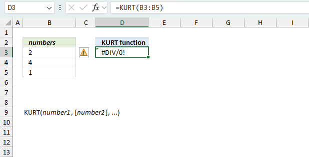
KURT returns the #DIV/0! error value:
- if there are fewer than four data points.
- if the standard deviation of the sample equals 0 (zero)
7.1 Troubleshooting the error value
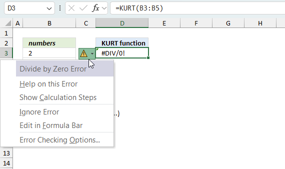
When you encounter an error value in a cell a warning symbol appears, displayed in the image above. Press with mouse on it to see a pop-up menu that lets you get more information about the error.
- The first line describes the error if you press with left mouse button on it.
- The second line opens a pane that explains the error in greater detail.
- The third line takes you to the "Evaluate Formula" tool, a dialog box appears allowing you to examine the formula in greater detail.
- This line lets you ignore the error value meaning the warning icon disappears, however, the error is still in the cell.
- The fifth line lets you edit the formula in the Formula bar.
- The sixth line opens the Excel settings so you can adjust the Error Checking Options.
Here are a few of the most common Excel errors you may encounter.
#NULL error - This error occurs most often if you by mistake use a space character in a formula where it shouldn't be. Excel interprets a space character as an intersection operator. If the ranges don't intersect an #NULL error is returned. The #NULL! error occurs when a formula attempts to calculate the intersection of two ranges that do not actually intersect. This can happen when the wrong range operator is used in the formula, or when the intersection operator (represented by a space character) is used between two ranges that do not overlap. To fix this error double check that the ranges referenced in the formula that use the intersection operator actually have cells in common.
#SPILL error - The #SPILL! error occurs only in version Excel 365 and is caused by a dynamic array being to large, meaning there are cells below and/or to the right that are not empty. This prevents the dynamic array formula expanding into new empty cells.
#DIV/0 error - This error happens if you try to divide a number by 0 (zero) or a value that equates to zero which is not possible mathematically.
#VALUE error - The #VALUE error occurs when a formula has a value that is of the wrong data type. Such as text where a number is expected or when dates are evaluated as text.
#REF error - The #REF error happens when a cell reference is invalid. This can happen if a cell is deleted that is referenced by a formula.
#NAME error - The #NAME error happens if you misspelled a function or a named range.
#NUM error - The #NUM error shows up when you try to use invalid numeric values in formulas, like square root of a negative number.
#N/A error - The #N/A error happens when a value is not available for a formula or found in a given cell range, for example in the VLOOKUP or MATCH functions.
#GETTING_DATA error - The #GETTING_DATA error shows while external sources are loading, this can indicate a delay in fetching the data or that the external source is unavailable right now.
7.2 The formula returns an unexpected value
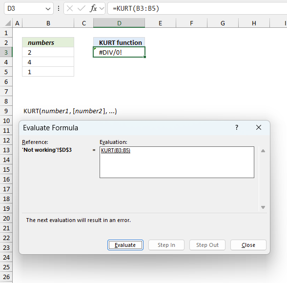
To understand why a formula returns an unexpected value we need to examine the calculations steps in detail. Luckily, Excel has a tool that is really handy in these situations. Here is how to troubleshoot a formula:
- Select the cell containing the formula you want to examine in detail.
- Go to tab “Formulas” on the ribbon.
- Press with left mouse button on "Evaluate Formula" button. A dialog box appears.
The formula appears in a white field inside the dialog box. Underlined expressions are calculations being processed in the next step. The italicized expression is the most recent result. The buttons at the bottom of the dialog box allows you to evaluate the formula in smaller calculations which you control. - Press with left mouse button on the "Evaluate" button located at the bottom of the dialog box to process the underlined expression.
- Repeat pressing the "Evaluate" button until you have seen all calculations step by step. This allows you to examine the formula in greater detail and hopefully find the culprit.
- Press "Close" button to dismiss the dialog box.
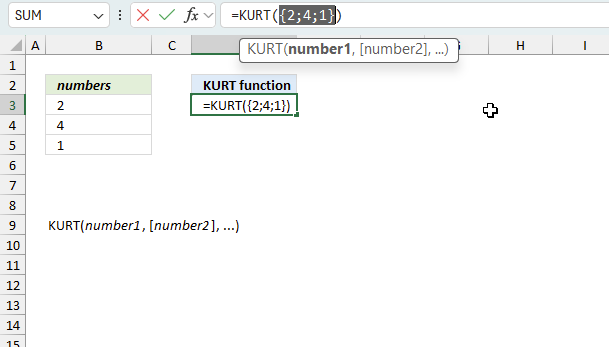
There is also another way to debug formulas using the function key F9. F9 is especially useful if you have a feeling that a specific part of the formula is the issue, this makes it faster than the "Evaluate Formula" tool since you don't need to go through all calculations to find the issue..
- Enter Edit mode: Double-press with left mouse button on the cell or press F2 to enter Edit mode for the formula.
- Select part of the formula: Highlight the specific part of the formula you want to evaluate. You can select and evaluate any part of the formula that could work as a standalone formula.
- Press F9: This will calculate and display the result of just that selected portion.
- Evaluate step-by-step: You can select and evaluate different parts of the formula to see intermediate results.
- Check for errors: This allows you to pinpoint which part of a complex formula may be causing an error.
The image above shows cell reference B3:B5 converted to hard-coded value using the F9 key. The KURT function requires at least 4 values in the argument which is not the case in this example. We have found what is wrong with the formula.
Tips!
- View actual values: Selecting a cell reference and pressing F9 will show the actual values in those cells.
- Exit safely: Press Esc to exit Edit mode without changing the formula. Don't press Enter, as that would replace the formula part with the calculated value.
- Full recalculation: Pressing F9 outside of Edit mode will recalculate all formulas in the workbook.
Remember to be careful not to accidentally overwrite parts of your formula when using F9. Always exit with Esc rather than Enter to preserve the original formula. However, if you make a mistake overwriting the formula it is not the end of the world. You can “undo” the action by pressing keyboard shortcut keys CTRL + z or pressing the “Undo” button
7.3 Other errors
Floating-point arithmetic may give inaccurate results in Excel - Article
Floating-point errors are usually very small, often beyond the 15th decimal place, and in most cases don't affect calculations significantly.
Useful resources
KURT function - Microsoft
Excel's KURT( ) function computes the excess kurtosis, not the kurtosis
How to Interpret Excess Kurtosis and Skewness
How to use the HARMEAN function 17 Apr 2023 11:17 PM (3 years ago)
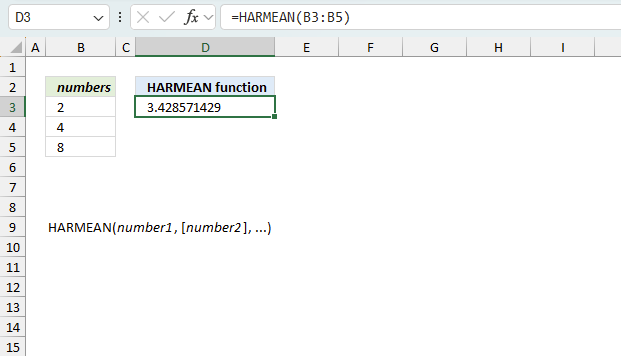
What is the HARMEAN function?
The HARMEAN function lets you calculate the harmonic mean in Excel.
Table of contents
1. Introduction
What is the harmonic mean?
The harmonic mean is a type of average that is useful for rates and ratios. It is calculated by taking the reciprocals of the values, averaging them, and reciprocating the result.
It gives more weight to smaller values compared to the arithmetic mean. The harmonic mean is useful when averaging rates and ratios instead of direct values.
The harmonic mean is always less than or equal to the arithmetic mean for a dataset. It is sensitive to small values which can skew or bias the average. Applications for the harmonic mean are averaging speed, fuel efficiency, ratios, and rates.
How is the harmonic mean calculated?
It is calculated by is calculated by dividing the number of values by the reciprocal of each value. For example, calculating the harmonic mean from numbers 2, 4, and 8 equals approx. 3.429
Here is how: 3/(1/2+1/4+1/8) equals approx. 3.429
To calculate the harmonic mean by hand use this formula:

H - harmonic mean
x1, x2, ..., xn - are the numbers
n is the number of values
What is the difference between the harmonic mean and the arithmetic mean (average)?
The difference between the harmonic mean and the arithmetic mean is that the harmonic mean is calculated by dividing the number of values by the reciprocal of each value, whereas the arithmetic mean is calculated by dividing the sum of all values by the number of values.
Divide 1 by the number to get the reciprocal of a number. Example the reciprocal of 4 is 1/4.
The AVERAGE function lets you calculate the arithmetic mean in Excel.
When to calculate the harmonic mean?
The harmonic mean is often the most useful measure for rates and ratios. It gives greater weight to smaller values in a given data set.
How is the weighted harmonic mean calculated?
The weighted harmonic mean is a variation of the regular harmonic mean that takes into account the relative weight of each data point. It is calculated using the following formula:
Weighted Harmonic Mean = n / Σ(wi / xi)
Where:
n is the sum of the weights (Σwi)
wi is the weight associated with each data point xi
xi is the value of the i-th data point
The steps to calculate the weighted harmonic mean are:
- Assign a weight (wi) to each data point (xi) based on their relative importance or significance.
- Calculate the reciprocal of each data point (1/xi).
- Multiply each reciprocal (1/xi) by its corresponding weight (wi).
- Sum up the weighted reciprocals from step 3: Σ(wi / xi)
- Calculate the sum of the weights: Σwi
- Divide the sum of the weights (Σwi) by the sum of the weighted reciprocals from step 4: n / Σ(wi / xi)
2. Syntax
HARMEAN(number1, [number2], ...)
3. Arguments
| Argument | Description |
| number1 | Required. A single numerical value or a cell reference to multiple numerical values. |
| [number2] | Optional. Up to 254 additional arguments. |
Text, logical values and empty cells are ignored.
The HARMEAN function returns
- #NUM! error value if number is less than or equal to 0 (zero).
4. Example 1

A manufacturing plant produces three different types of components. The production rates (units per hour) for each type are as follows: Type A: 50, 60, 70 Type B: 45, 55, 65 Type C: 40, 50, 60 Calculate the harmonic mean of the production rates for each type of component?
The image above shows the production rates in cell range B15:F18, the column chart shows the different production rates grouped in category A, B and C.
Formula in cell F16:
The formula in cell F16 calculates the harmonic mean based on the following production rates: 50, 60, and 70. The calculation is 3/(1/50+1/60+1/70) equals approx 58.88
The formula in cell F17 returns the harmonic mean based on these production rates: 45, 55, and 65. The calculation is 3/(1/45+1/55+1/65) equals approx 53.77
The formula in cell F18 returns the harmonic mean based on these production rates: 40, 50, and 60. The calculation is 3/(1/40+1/50+1/60) equals approx 48.65
5. Example 2

A car travels at 10 mph (miles per hour) for 1 mile, 30 mph for 5 miles, and 50 mph for 2 miles. The total distance is 8 miles. What is the average speed?
The formula for calculating the distance: Distance = Speed x Time
This gives us: Speed = Distance / Time
The total distance is 1 + 5 + 2 equals 8.
The time it takes to travel a distance is calculated like this:
Time = Distance / Speed
The harmonic weighted average is (1+5+2)/(1/10 + 5/30 + 2/50)
becomes 8/(23/75)
equals approx. 26.09 mph.
Weighted harmonic average formula in cell F4:
The formula in cell F4 returns approx. 26.09 which matches the calculated value we did above.
Explaining formula
Step 1 - Add distances
The SUM function allows you to add numerical values, the function returns the sum in the cell it is entered in. The SUM function is cleverly designed to ignore text and boolean values, adding only numbers.
Function syntax: SUM(number1, [number2], ...)
SUM(C3:E3) becomes SUM({1,5,2}) and returns 8.
Step 2 - Divide distance with speed
The division character lets you calculate a ratio based on a numerator and denominator..
C3:E3/C4:E4 becomes {1,5,2}/{10,30,50} and returns {0.1,0.166666666666667,0.04}
Step 3 - Add ratios and return a total
SUM(C3:E3/C4:E4) becomes SUM({0.1,0.166666666666667,0.04} and returns 0.306666666666667
Step 4 - Divide total distance by total time
SUM(C3:E3)/SUM(C3:E3/C4:E4)
becomes
8/0.306666666666667
and returns 26.0869565217391
6. Example 3

A manufacturing plant produces electronic components. The production rates (units per hour) are 50 units/hour while producing 275 units, 25 units/hour for 120 units, 10 units/hour for 435 units, and 40 units/hour for 10 units. What is the average production rate, in other words, calculate the weighted harmonic mean of the production rates?
Cell range B16:C20 contains a data table with the following header names: "Production rate (units/hour)" and "Units produced".
| Production rate (units/hour) |
Units produced |
| 50 | 275 |
| 25 | 120 |
| 10 | 435 |
| 40 | 10 |
Formula in cell C22:
The formula in cell C22 calculates the weighted harmonic mean based on the data in B17:C20. The result is approx. 15.54 units/hour.
7. Function not working
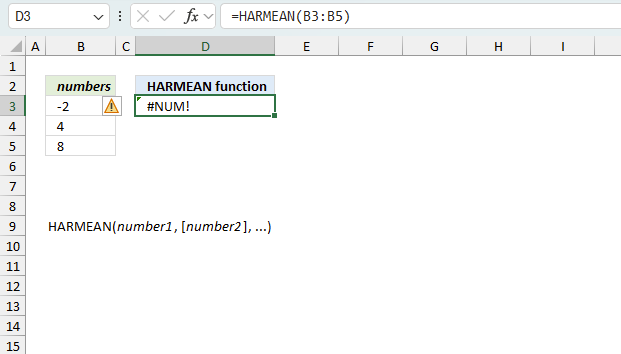
When an array or reference argument contains text, logical values, or empty cells, they are disregarded in the calculation, but cells containing the value zero are taken into account. Arguments that are error values or text that cannot be translated into numbers cause errors.
HARMEAN returns the #NUM! error value if any data point ≤ 0
7.1 Troubleshooting the error value
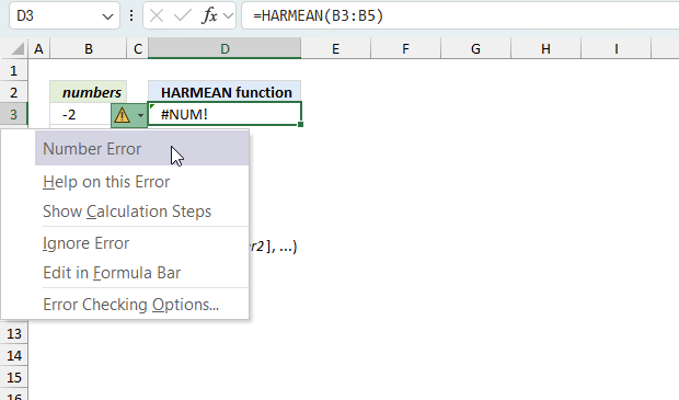
When you encounter an error value in a cell a warning symbol appears, displayed in the image above. Press with mouse on it to see a pop-up menu that lets you get more information about the error.
- The first line describes the error if you press with left mouse button on it.
- The second line opens a pane that explains the error in greater detail.
- The third line takes you to the "Evaluate Formula" tool, a dialog box appears allowing you to examine the formula in greater detail.
- This line lets you ignore the error value meaning the warning icon disappears, however, the error is still in the cell.
- The fifth line lets you edit the formula in the Formula bar.
- The sixth line opens the Excel settings so you can adjust the Error Checking Options.
Here are a few of the most common Excel errors you may encounter.
#NULL error - This error occurs most often if you by mistake use a space character in a formula where it shouldn't be. Excel interprets a space character as an intersection operator. If the ranges don't intersect an #NULL error is returned. The #NULL! error occurs when a formula attempts to calculate the intersection of two ranges that do not actually intersect. This can happen when the wrong range operator is used in the formula, or when the intersection operator (represented by a space character) is used between two ranges that do not overlap. To fix this error double check that the ranges referenced in the formula that use the intersection operator actually have cells in common.
#SPILL error - The #SPILL! error occurs only in version Excel 365 and is caused by a dynamic array being to large, meaning there are cells below and/or to the right that are not empty. This prevents the dynamic array formula expanding into new empty cells.
#DIV/0 error - This error happens if you try to divide a number by 0 (zero) or a value that equates to zero which is not possible mathematically.
#VALUE error - The #VALUE error occurs when a formula has a value that is of the wrong data type. Such as text where a number is expected or when dates are evaluated as text.
#REF error - The #REF error happens when a cell reference is invalid. This can happen if a cell is deleted that is referenced by a formula.
#NAME error - The #NAME error happens if you misspelled a function or a named range.
#NUM error - The #NUM error shows up when you try to use invalid numeric values in formulas, like square root of a negative number.
#N/A error - The #N/A error happens when a value is not available for a formula or found in a given cell range, for example in the VLOOKUP or MATCH functions.
#GETTING_DATA error - The #GETTING_DATA error shows while external sources are loading, this can indicate a delay in fetching the data or that the external source is unavailable right now.
7.2 The formula returns an unexpected value
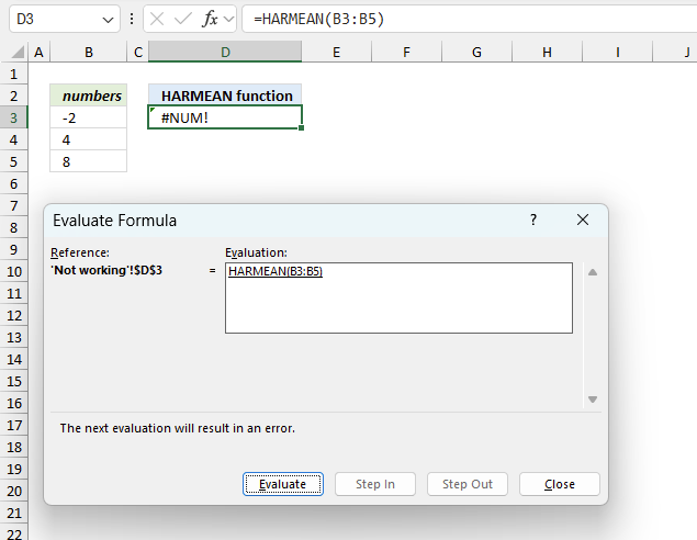
To understand why a formula returns an unexpected value we need to examine the calculations steps in detail. Luckily, Excel has a tool that Here is how to troubleshoot a formula:
- Select the cell containing the formula you want to examine in detail.
- Go to tab “Formulas” on the ribbon.
- Press with left mouse button on "Evaluate Formula" button. A dialog box appears.
The formula appears in a white field inside the dialog box. Underlined expressions are calculations being processed in the next step. The italicized expression is the most recent result. The buttons at the bottom of the dialog box allows you to evaluate the formula in smaller calculations which you control. - Press with left mouse button on the "Evaluate" button located at the bottom of the dialog box to process the underlined expression.
- Repeat pressing the "Evaluate" button until you have seen all calculations step by step. This allows you to examine the formula in greater detail and hopefully find the culprit.
- Press "Close" button to dismiss the dialog box.
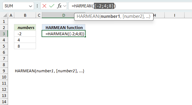
There is also another way to debug formulas using the function key F9. F9 is especially useful if you have a feeling that a specific part of the formula is the issue, this makes it faster than the "Evaluate Formula" tool since you don't need to go through all calculations to find the issue..
- Enter Edit mode: Double-press with left mouse button on the cell or press F2 to enter Edit mode for the formula.
- Select part of the formula: Highlight the specific part of the formula you want to evaluate. You can select and evaluate any part of the formula that could work as a standalone formula.
- Press F9: This will calculate and display the result of just that selected portion.
- Evaluate step-by-step: You can select and evaluate different parts of the formula to see intermediate results.
- Check for errors: This allows you to pinpoint which part of a complex formula may be causing an error.
The image above shows cell reference B3 converted to hard-coded value using the F9 key. The HARMEAN function requires a number larger than or equal to 0 (zero) which is not the case in this example. We have found what is wrong with the formula.
Tips!
- View actual values: Selecting a cell reference and pressing F9 will show the actual values in those cells.
- Exit safely: Press Esc to exit Edit mode without changing the formula. Don't press Enter, as that would replace the formula part with the calculated value.
- Full recalculation: Pressing F9 outside of Edit mode will recalculate all formulas in the workbook.
Remember to be careful not to accidentally overwrite parts of your formula when using F9. Always exit with Esc rather than Enter to preserve the original formula. However, if you make a mistake overwriting the formula it is not the end of the world. You can “undo” the action by pressing keyboard shortcut keys CTRL + z or pressing the “Undo” button
7.3 Other errors
Floating-point arithmetic may give inaccurate results in Excel - Article
Floating-point errors are usually very small, often beyond the 15th decimal place, and in most cases don't affect calculations significantly.